Common Cause Failures (CCF) would indicate the failures of multiple components in a system due to some cause. In this paper, an attempt has been made to analyze the Limiting State Probabilities (LSP) of states for small repairable systems in which, the components are prone for failures due to CCF. For large systems, the same can also be used, as failure modes represent cut sets of the system and it is known that cut sets of order more than three can be ignored as they don't contribute much to predict the indices for approximate system reliability analysis. Analysis of repairable components with CCF is presented with a case study.
In general, component failures can be of two types,
1) Catastrophic (or) Permanent failures, and
2) Repairable components.
CCF [5,12] are failures in which a single error or problem disables multiple, independent safety functions. A CCF is a dependent failure in which two or more component fault states exist within a short interval or simultaneously due to a shared cause. [13, 15, 18] CCF can occur owing to common external or internal influences. External causes may involve operational, environmental or human factors. Internal causes may involve manufacturing defects, aging effects, etc. Fault models for CCF in redundant systems are developed and techniques to design redundant systems protected against the modelled CCF are implemented [5]. Heterogeneous redundancy optimization for multi-state series–parallel systems subject to Common Cause Failures is proposed in [10]. A method for reliability modelling and assessment of a multi-state system with CCF is proposed in [11,14].
CCF analysis of a two non-identical unit parallel system with arbitrarily distributed repair times is proposed in [1]. An expression for the Mean Time To Failure, MTTF k/n, of a non repairable k out of n:G identical unit system with warm standby and CCF is presented in [3].
Generalized expression for MTTF of a non repairable identical unit parallel system with warm standby and CCF is developed in [2]. Time varying failure rates and Markov chain analysis are combined to obtain a hybrid reliability and availability analysis [4]. A stochastic analysis of a non identical two unit parallel system with CCF by graphical evaluation and review techniques is presented in [7] .
A method for analyzing availability and reliability of repairable systems with CCF among components is proposed in [6]. Exponential asymptotic property of a parallel repairable system with CCF is explored [8]. Availability and Reliability analysis of a k-out-of-(M+S): G warm standby system with repair and time varying failure rates in the presence of CCF is presented [9].
In this paper, the effects of CCF are considered for 2- component repairable system with identical/Nonidentical transitional rates with 4-state and 5-state models. It is extended to a 3-component repairable system which includes CCF. In this Paper, analysis with CCFs and repairable components is presented with practical case study. Case study with Load-Node scheme has been considered in [16], the data is obtained from [17] and the analysis using cut sets is carried out in this paper. Section 1 provides the objective of the paper. Section 2 provides the proposed methodology to find the Stochastic Transitional Probability Matrix (STPM) for 2 component, 3 component repairable systems with CCF have been considered and expressions for LSP have been derived for 4 state and 5 state models. A sample power distribution network is considered in section 3 and the results are compared with components with and without CCF in section 4. Finally, the paper is concluded.
The objective in this section is to find the LSP of the states of two component and three component systems.
Consider two component repairable system with nonidentical transition rates and non-identical capacities wherein due to CCF are occurring, the Complete State Space Diagram (CSSD) can be shown in two ways,
(a) 4 State Model:
The CSSD of a two component system when repairable components when CCF can occur will be shown in Figure 1 [13].
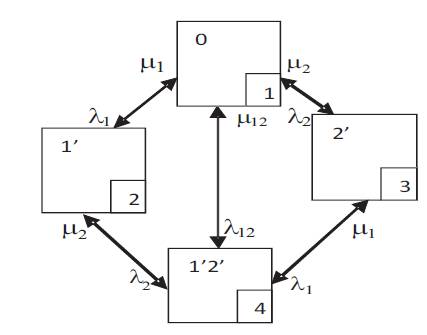
Figure 1. CSSD of a Two Component Repairable System with CCF
where λ1,λ2 and µ1,µ2 are the failure rates and repair rates of components 1 and 2 respectively. λ12 is the failure rate of both components 1, 2 due to common cause and µ12 is the repair rate of both components simultaneously so that the system can transit from state 4 to state 1 directly.
The STPM can be obtained as:
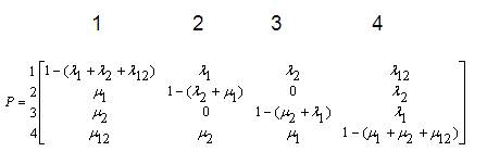
The objective will be to find the LSP of the states in Figure1, using LSP vector approach.
Let α be the LSP vector = [ P1 P2 P3 P4 ]
where P1 , P2 , P3 , P4 are the LSP of states 1 to 4 respectively in Figure 1.
The solution methodology is :
α P = α
[P1 P2 P3 P4].
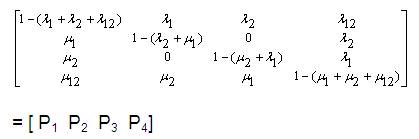
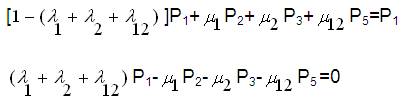
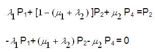
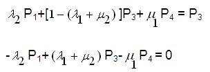
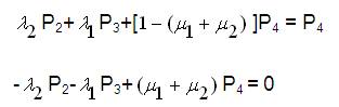
Now expanding equation (2),
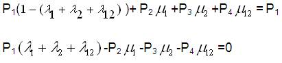
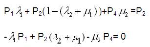
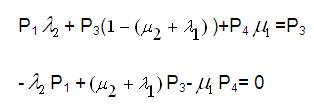
Since the equations deduced from equation (2) will be having only three linearly independent equations and the other one shall be,
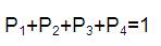
Writing equations (3) to (6) in matrix form,
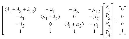
Although in the earlier methods, Cramer's rule has been shown to be adopted for solving P1 , P2 , P3 , P4 , for higher number of variables, Cramer's rule becomes cumbersome and laborious. The advantage of equation (7) is that the values of LSP will be finite and lies between zero and one and therefore the set of linear algebraic equations have a unique solution. Therefore, Gauss elimination method or Gauss Jordon method can be used for solving P1 , P2 , P3 , P4 if the data is known.
Now, if the components or units have identical capacities and identical transitional rates, Figure 1 can be reduced to Figure 2.
Now, the STPM can be written as,
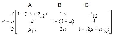
Figure 2 shows the Merged State Space Diagram (MSSD) of a two component repairable system with CCF.
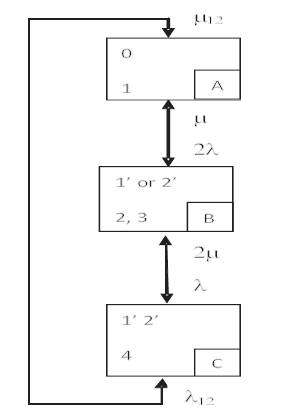
Figure 2. Merged State Space Diagram (MSSD) of a Two Component Repairable System with CCF
The objective will be to find the LSP of the states in Figure 2 using LSP vector approach.
Let α be the LSP vector = [ PA PB PC ],
where PA , PB , PC are the LSP of states A to C respectively in Figure 2.
Now the solution methodology is,
αP = α
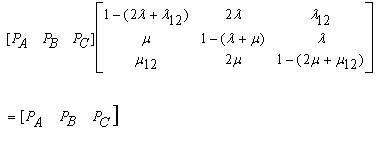
Now expanding equation (9),
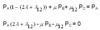
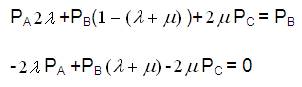
and the other equation will be:
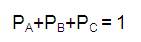
Writing equations (10) to (12) in matrix form
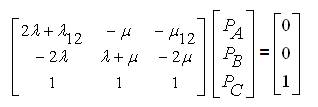
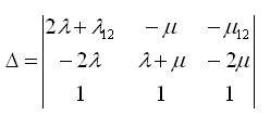
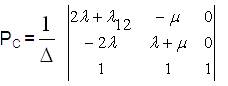
Solving equation (13) using Cramer's rule,
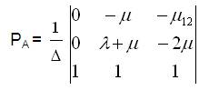
where
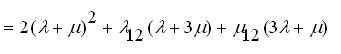
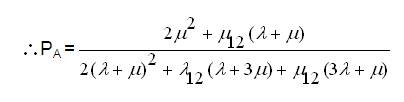
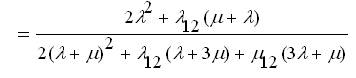
Now

Now
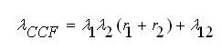
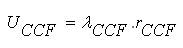
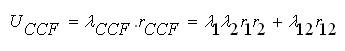
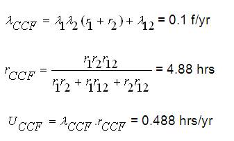
Now, the equivalent failure rate of the components including CCF for 4 state model can be expressed as [13],
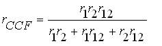
The mean outage time can be expressed as,
The average annual outage time can be expressed as,
(b) 5 - State Model:
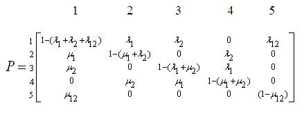
The CSSD of a two component system when repairable components due to CCF can occur with 5 –state model is shown in Figure 3 [13].
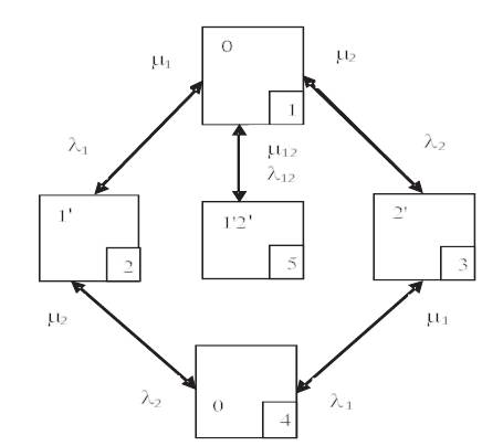
Figure 3. CSSD of a Two Component Repairable System with CCF as 5-state Model
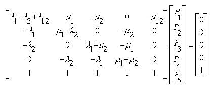
The STPM can be obtained from Figure 3 as:
Now, the objective will be to find the LSP of the states 1 to 5 in Figure 3, using LSP vector approach.
Let α be the LSP vector = [P1 P2 P3 P4 P5 ]
where, Pi i = 1 to 5, is the LSP of state 'i’.
Figure 3 shows the CSSD of a two component repairable system with CCF as 5-state model
The solution methodology is : α P = α
[P1 P2 P3 P4 P5 ].
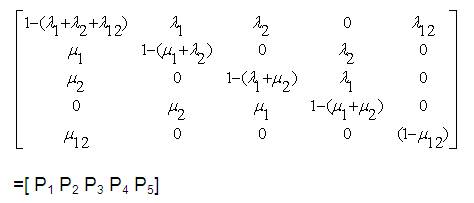
Now expanding Equation (21),
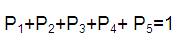
Since the equations deduced from equation (21) will be having only four linearly independent equations and the other one shall be,
Now writing equations (22) to (26) in matrix form,
As stated in the previous section, Gauss - elimination method or Gauss - Jordon method can be used for solving P1 , P2 , P3 , P4 and P5 .
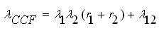
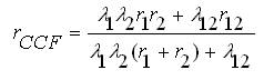
Now the equivalent failure rate of the components including CCF for 5 state model can be expressed as [13],
The mean outage time can be expressed as,
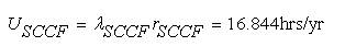
The average annual outage time can be expressed as,
For example, consider that there are two components in a system having failure rates of 0.125 f/yr, 0.2 f/yr respectively, and repair times of 14 hrs and 12 hrs respectively. The failure rate and repair time due to CCF of the components will be 0.1 f/yr and 20 hrs respectively.
The Basic Probability Indices for the system can be calculated as follows,
i) With no CCF:
λ1 = 0.125 f/yr; λ2 = 0.2 f/yr; λ12 = 0; r12 = 0
r1 = 14 hrs; r2 = 12 hrs
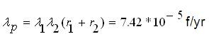
The equivalent failure rate of the system is,
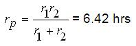
The mean outage time of the system is,
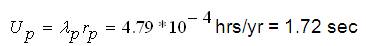
The average annual outage time is,
ii) With CCF of 4 State Model
Here λ12 = 0.1 f/yr; r12 = 20 hrs
iii) With CCF of 5 State Model
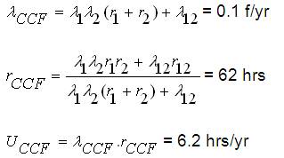
Figure 4 shows the CSSD of a three component repairable system with CCF as 8-state model. Consider three component repairable system with non-identical transition rates and non- identical capacities wherein due to CCF are occurring, the CSSD can be shown in Figure 4 with 8 – state model.
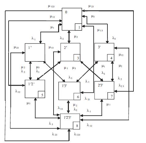
Figure 4. CSSD of a Three Component Repairable System with CCF as 8-state Model
If the components or units have identical capacities, then Figure 4 can be reduced to 4 state model if the states 2, 3, 4 and 5, 6, 7 are merged as shown in Figure 5, and let λ1=λ2=λ3=λ; µ1=µ2=µ3=µ.
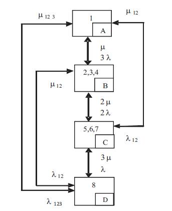
Figure 5. MSSD of a Three Component Repairable System with CCF having Identical Capapcities and Transition Rates
The STPM can be obtained from Figure 5 as,
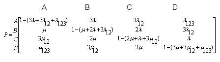
Now, the objective will be to find the LSP of the states A, B, C and D in Figure 5.
Let α be the LSP vector = [PA PB PC PD ]
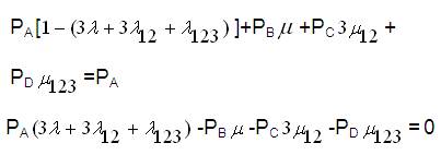
where 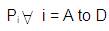 , is the LSP of state 'i'
Now the solution methodology is : αP = α
[PA PB PC PD ].
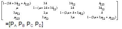
Now expanding equation (32),
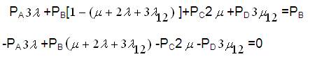
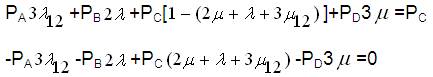
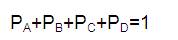
Since the equations deduced from equation (32) will be having only three linearly independent equations and the other one shall be,
Writing equations (33) to (36) in matrix form,
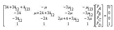
As stated in the previous section, Gauss - elimination method or Gauss - Jordon method can be used for solving PA , PB , PC and PD .
The Load Node scheme is shown in Figure 6. Two fully redundant HV/MV transformer bays feed the two relevant MV bus-bars. The components considered are Circuit Breakers, Transformers, and Feeders. It has to be stated that, the Circuit Breaker duty is to clear faults on other equipment, but itself can be subject to fault. It can also be stated that, there is a possibility of CCF in case of a failure on a transformer, due to the possible overload of the other transformer. It is considered that the failure modes of the first failure and CCF are different. The first failure can be an internal fault, conversely the CCF is due to an overload that can be caused by a design under-sizing. Failure and repair times of Load Node scheme are given in Table 1 [16,17].
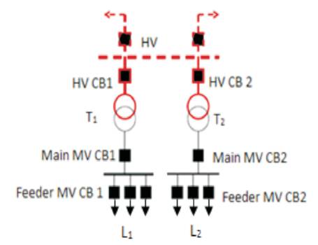
Figure 6. Load Node Scheme
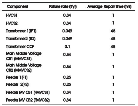
Table 1. Failure and Repair Times of Load-Node Scheme
The Reliability Logic Diagrams (RLD) for load groups L1 , L2 and Load Node scheme using cut sets are shown in Figures 7 and 8 respectively.
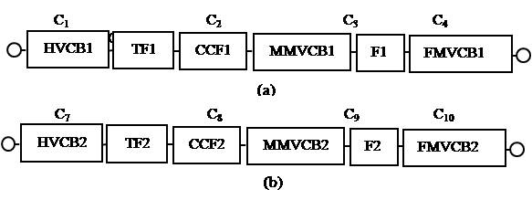
Figure 7. RLD for (a) Load Group L1 (b) Load Group L2
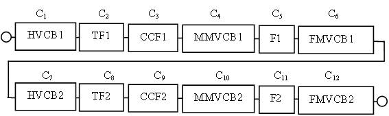
Figure 8. RLD of Load-Node Scheme using Cut sets
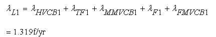
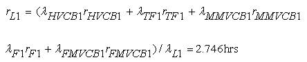
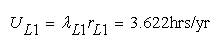
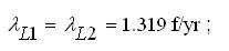
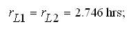
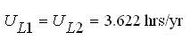
The Basic Probability Indices (BPI) of Load group 1 (L1 ) without CCF are obtained as,
As identical components are considered, the BPI of Load group 2 (L2 ) without CCF are given as,
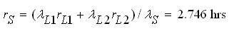
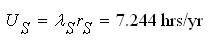
The BPI of Load-Node scheme without CCF are obtained as,

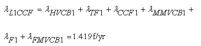
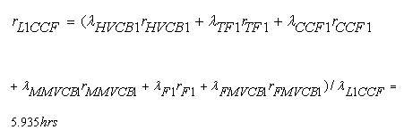
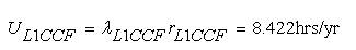
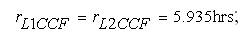
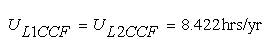
The BPI of Load group 1 (L1) with CCF are obtained as,
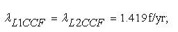
As identical components are considered, the BPI of Load group 2 (L2 ) with CCF are given as,
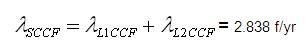
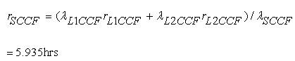
The BPI of Load-Node scheme with CCF are obtained as,
Thus, the BPI obtained with and without CCF are presented in Table 2. From Table 2, it can be observed that equivalent failure rate, repair time and average annual outage time will increase with CCF for Load groups L1 , L2 and for the system as well.
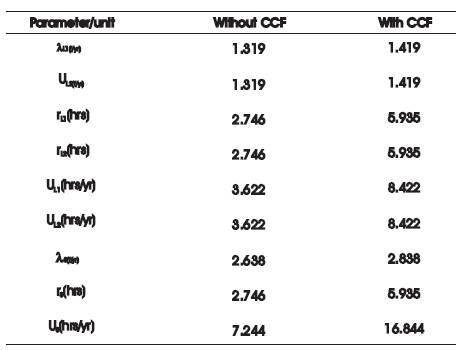
Table 2. Basic Probability Indices with and without CCF
In this paper, the concept of Common Cause Failures has been discussed. For repairable components, the analysis using CCF has been dealt by considering two component and three component repairable models. It can also be extended to nine state model of a three component system. A study is carried out on a power distribution network, and the results are presented for the component probabilities with and without CCF. It is concluded that, all the Basic Probability Indices will be increased with increase in Common Cause Failure rates of the components in the system and from the feeder to the corresponding load points also.