Round Robin (RR) scheduling algorithm is a widely used scheduling algorithm in timesharing systems, as it is fair to all processes and is free of starvation. The performance of the Round Robin algorithm depends very much on the size of the time quantum selected. If the time quantum is too large, the performance of the algorithm would be similar to that of FCFS (First Come First Serve) scheduling. On the other hand, if the time quantum is too small, the number of context switches will be large. Therefore, it is necessary to have some idea about the optimum level of time quantum, so that the average waiting time and turnaround times, and the number of context switches are not too large. Several extensions to the round robin algorithm have been proposed in the literature to overcome these difficulties. In this study, the author has picked some of these extensions and tried comparing their effectiveness by means of some examples.
Round Robin (RR) is a scheduling algorithm designed especially for time sharing systems. It is somewhat similar to FCFS scheduling. The difference is that in RR, preemption of processes is allowed while there is no preemption in FCFS scheduling. When preemption of processes is allowed, a process is interrupted before completion, and the balance part is implemented in later stages. The idea is to give a fair share of processing to each available process.
In RR scheduling, a small time unit, known as a time quantum is defined, which is considered as the time limit allowed for each process at a time. The ready queue of processes is considered as a circular queue. Once a process spent its time quantum, it is preempted, which means that the process is interrupted and the remaining part is moved to the end of the queue using a context switch. Then, the next process takes over. This procedure continues until all the processes are completed. However, when a process completes its execution before its allocated time quantum is over, the next process in the ready queue continues execution.
Even though this idea may be attractive and looks fair for all the processes, it has its drawbacks as well. In fact, the performance of the RR algorithm depends very much on the size of the time quantum selected. If the time quantum is too large, the performance of the algorithm would be similar to that of FCFS scheduling. On the other hand, if the time quantum is too small, the number of context switches will be large. Therefore, it is necessary to have some idea about the optimum level of time quantum so that, the number of context switches would be limited and at the same time, average waiting time and turnaround times are not too large. Waiting time is the amount of time, a process spends waiting in the ready queue. The interval from the time of submission of a process at the time of completion is the turnaround time.
The paper is organized as follows : In section 1, the author presents some related work which extends the Round Robin scheduling concept. In section 2, the author discuss the computational experience by illustrating the detailed calculations. The author compares the performance of the algorithms in section 3, and the last section concludes the paper.
A number of algorithms has been proposed to improve the outcome of the Round Robin scheduling. It is assumed that, the burst time of each process in the queue is known. Burst time is the actual time that is required to complete execution of a particular process or task in the computer. Instead of the static time quantum, a dynamic time quantum has been proposed by some of these approaches. However, in most of these, only examples of small sizes have been used to illustrate these procedures. The other problem is that, in most of these approaches, sorting the burst times of the given processes is required before hand, which might affect the speed of computation when a large number of processes are present in a given list. Therefore, the validity of these claims could not be verified for larger size problems as theoretical proofs have not been provided.
Here, a summary of each algorithm has been presented that the author has compared in this study. Certain algorithms were not mentioned as they give rise to very similar results.
In addition, several other algorithms have also been proposed to solve this problem.
An algorithm presented by Kundargi and Emmi (2014) attempts to improve the disadvantage of Round Robin algorithm by using a dynamic time quantum.
Jaiswal et al. (2013) have proposed an approach on a dynamic time quantum, which is repeatedly changed to the immediate greater value of the previous time quantum.
Mishra and Rashid (2014) has presented an algorithm in which the dynamic time quantum is repeatedly adjusted to the minimum value of retaining burst time.
Datta et.al. (2015) have proposed an algorithm based on Round Robin and the shortest job first scheduling. Khankasikam (2013) has proposed an algorithm in which the time quantum is repeatedly adjusted according to the burst time of the running processes.
Helmy and Dekdouk (2007) has proposed an algorithm based on a weighting technique as an attempt to combine the low scheduling overhead of round robin algorithms and favor short jobs.
Most of the papers mentioned above have illustrated their algorithms using small size examples such as problems with only five processes. Therefore, the author has randomly generated problems containing more processes (eg. using 7 and 12 processes) in order to study the behavior of these algorithms. The programs for the basic Round Robin algorithm and the eight extensions of the algorithm were tested using the same set of examples. The programs were implemented with a simulator constructed using a Pascal compiler.
The detailed computational steps are presented with respect to all the algorithms considered using the problem with 7 processes as given below. A summary of results for a 12 process problem is also presented in the next section.
Example 1:
Problem with 7 processes
Burst time: 30, 15, 45, 85, 20, 32, 18
Total burst time = 245
Average burst time = 245/7 = 35
An arbitrary time quantum of 30 has been used in the round robin algorithm. Implementation of Round Robin algorithm is shown in Table 1.
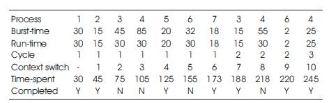
Table 1. Implementation of Round Robin Algorithm (Time Quantum = 30)
Total turnaround time = 30+45+ 188 + 245 + 125 + 220 + 173 = 1026
Average turnaround time = 1026/7 = 146.6
Total waiting time = 1026 – 245 = 781
Average waiting time = 781/7 = 111.6
Context switches = 10
An arbitrary time quantum of 30 has been used for the improved RR algorithm (Ahad, 2012). A threshold value k is added to the time quantum whenever it is possible to finish a process without preemption. K is the ceiling (x), where x is the average left out time of uncompleted processes. Left out time is the remainder, when the burst time of each process is divided by the time quantum where the burst time is greater than the time quantum, Therefore, the left out times for the given processes are 0, 0, 15, 25, 0, 2, 0.
Hence, k = ceiling ( 15+25+2/7) = ceiling ( 42/7) = ceiling (6) = 6
Therefore, even though the time quantum is 30, whenever it is possible to complete a process, a time quantum of 36 could be used. Table 2 shows the implementation of improved RR algorithm.
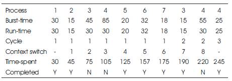
Table 2. Implementation of Improved RR Algorithm (Time Quantum = 30, k = 6)
Total turnaround time = 30+45+190+245 +125+157+ 175 = 967
Average turnaround time = 967/7 = 138.1
Total waiting time = 967 – 245 = 722
Average waiting time = 722/7 = 103.1
Context switches = 8
Time quantum = average of burst times of all processes = 245/7 = 35
Implementation of DTQRR algorithm is shown in Table 3 (Barman, 2013).
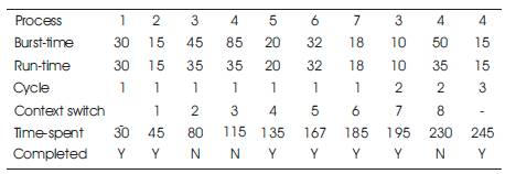
Table 3. Implementation of DTQRR Algorithm
Total turnaround time = 30+45+195+245+135+167+ 185 = 1002
Average turnaround time = 1002/7 = 143.1
Total waiting time = 1002 – 245 = 757
Average waiting time = 757/7 = 108.1
Context switches = 8
Two time quanta are used according to this algorithm. First, the processes are arranged according to the ascending order of burst times. Accordingly, the median of burst times is 30, which is the fourth burst time in the ascending order. This time quantum is used up to the fourth burst time in the list. The time quantum taken for the remaining processes from the next process in the queue is the upper quartile, which is 45 (Behera 2011). Implementation of MTDQRR algorithm is shown in Table 4.
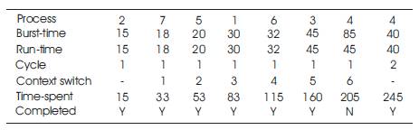
Table 4. Implementation of MTDQRR Algorithm
Total turnaround time =15+33+53+83+115+160+245 = 704
Average turnaround time = 704/7 = 100.6
Total waiting time = 704 – 245 = 459
Average waiting time = 459/7 = 65.6
Context switches = 6
In this algorithm, the median of remaining burst times are adjusted repeatedly. Here, the time quantum is dynamic and taken as the median burst time. However, if the median is less than 25, it is taken equal to 25. Initially, the time quantum is set at 30, which is the median of burst times of the processes in the queue. After the first cycle, processes 6, 3 , and 4 still remain to be completed. The median for these processes is 15, which is less than 25. Therefore, according to the algorithm, time quantum is taken as 25 for the remaining processes. After that, only the process 4 goes to the third cycle (Matanech 2009) .
Table 5 shows the SARR algorithm implementation.
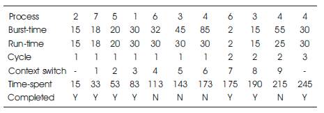
Table 5. Implementation of SARR Algorithm
Total turnaround time =15+33+53+83+175+190+245 = 794
Average turnaround time = 794/7 = 113.4
Total waiting time = 794 – 245 = 549
Average waiting time = 549/7 = 78.4
Context switches = 9
An arbitrary time quantum of 30 is used in this example. A threshold value is equal to one-fourth of the time quantum, which is equal to 8 is considered here. This threshold value is added to the time quantum, whenever it is possible to complete a particular process without preemption (Negi 2013). CRR algorithm is shown in Table 6.
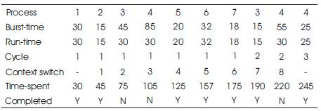
Table 6. Implementation of Conventional RR Algorithm
Total turnaround time = 30+45+190+245+125+157+ 175 = 967
Average turnaround time = 967/7 = 138.1
Total waiting time = 967 – 245 = 722
Average waiting time = 722/7 = 103.1
Context switches = 8
Initially, the time quantum is taken as the burst time of the first process in the queue. Afterwards, the time quantum is modified and taken as the average of remaining burst times in the queue. Hence, the initial time quantum is 30. Subsequent time quanta are 24 and 31 (Noon 2011). Implementation of AN algorithm is shown in Table 7.
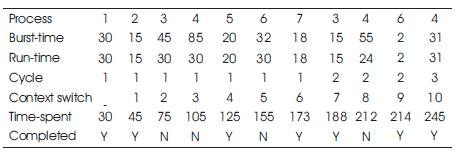
Table 7. implementation of AN Algorithm
Total turnaround time = 30+45+188+245+125+214+ 173 = 1020
Average turnaround time = 1020/7 = 145.7
Total waiting time = 1020 – 245 = 775
Average waiting time = 775/7 = 110.7
Context switches = 10
Initially, the time quantum is taken as the floor (x), where x is the average of the burst times of the processes in the queue which is 35 in this example. Processes with burst times less than or equal to the time quantum are executed according to the basic round robin algorithm. Then, the processes with burst times exceeding the time quantum are arranged according to the remaining burst times and the number of cycles and allocate CPU. If the remaining burst time of current process is less than one time quantum, allocate CPU again to the current process. Otherwise, go to the next process (Rao 2015). Table 8 shows the Implementation of CRR algorithm.
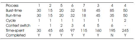
Table 8. implementation of Improved CRR Algorithm
Total turnaround time = 30+45+65+97+115+160+245 = 757
Average turnaround time = 757/7 = 108.1
Total waiting time = 757 – 245 = 512
Average waiting time = 512/7 = 73.1
Context switches = 6
In this algorithm, Vijaya Lakshmi (2015) calculated the time quantum as follows (Table 9).
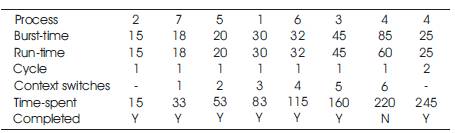
Table 9. Implementation of RR Scheduling Algorithm
Time quantum = (max. burst time-min. burst time)x median/average burst time.
= (85-15) x 30/35 = 60
Total turnaround time = 15+33+53+83+115+160+ 245 = 704
Average turnaround time = 704/7 = 100.6
Total waiting time = 704 – 245 = 459
Average waiting time = 459/7 = 65.6
Context switches = 6.
The author has compared the performance of the above algorithms based on the standard criteria: average turn around time, average waiting time and the number of context switches. In order to compare them, the author has used two numerical examples, one containing 7 processes and another problem with 12 processes.
Results are presented in Tables 10 and 11. RR indicate the results obtained for the standard Round Robin algorithm.
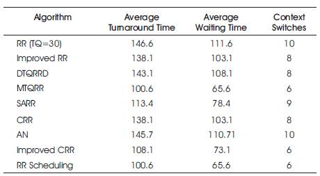
Table 10. Comparison of Algorithms for Example Problem with 7 Processes
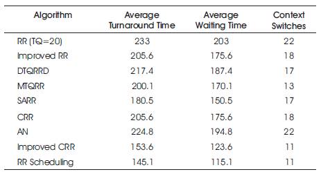
Table 11. Comparison of Algorithm for Example Problem with 12 Processes
Example 1: problem with 7 processes
Burst times: 30, 15, 45, 85, 20, 32, 18
Example 2: problem with 12 processes.
Burst times:15,40,18,25,68, 30,22, 42,10,16,35,39
From the above results, it can be seen that, out of the eight algorithms compared with the Round Robin algorithm, results obtained from the four algorithms appeared to be superior than those of the others. These are the algorithms proposed by Behera (2011), Matanech (2009), Rao et. al. (2015), and Vijaya Lakshmi (2015). Algorithms proposed by Negi (2013), Ahad (2012), Barman (2013), and Noon (2011) are placed lower down the order according to the results obtained from the example problems. However, it is not possible to rank them according to the superiority without considering further examples.
An advantage of the algorithm proposed by Behera et. al. (2011) was that, the time quantum is calculated twice in a single Round Robin cycle. First, the median of the burst time is taken as the time quantum up to the process considered as the median. For the succeeding processes, the time quantum is determined by taking the burst time of Upper Quartile of all the processes. This helps to reduce the overall processing time.
In the algorithm proposed by Mataneh (2009), the median of remaining burst time is adjusted repeatedly. This can be considered as a strength of this algorithm. Here, the time quantum is dynamic and is taken as the median burst time.
The benefit of the algorithm proposed by Rao et. al. (2015) is that, time slices of only those processes which require a slightly greater time slice than the allotted time cycles are only modified.
A strength of the algorithm presented by Vijaya Lakshmi (2015), is that a formula has been used to determine the time quantum. It attempts to define the finest time quantum using a formula which incorporate maximum, minimum and median burst times.
An advantage of the conventional RR (Negi 2013) algorithm is that, a threshold value is added to the time quantum, whenever it is possible to complete a particular process without preemption. However, a drawback of this algorithm is that, an arbitrary time quantum has to be used in solving a given problem.
A special feature of the improved RR (Ahad 2012) algorithm is that, the processes waiting in the ready queue are divided into two categories. The processes in the first category are the one for which the time quantum is modified and the processes in the second category will be processed as per the classical Round Robin algorithm. This algorithm also suffers from the necessity to use an arbitrary time quantum.
Noon et al. (2011) proposed an algorithm in which, initially, the time quantum is taken as the burst time of the first process in the queue. However, no justification was made for this selection: whether this approach would improve the performance of the algorithm.
The time quantum is set to be the average of burst time of all the processes in the algorithm proposed by Barman (2013) . However, it was not mentioned whether this method would improve the performance of the algorithm.
In the absence of any theoretical results to establish the superiority of a particular algorithm, it is difficult to generalize the results that the author has obtained. However, in order to further generalize these results, problems with a much larger number of processes need to be solved.
But, based on the results that the author has already obtained, out of the eight algorithms tested, four algorithms stand clearly above the other algorithms in the list. These are the algorithms proposed by Vijaya Lakshmi (2015), Rao et al. (2015), Matanech (2009), and Behera (2011). However, all of these papers report their results and analyze them based on the examples of small size containing few processes only. Hence, it is not possible to rank them according to the level of performance. Therefore, it is necessary that, more comprehensive analysis of the performance of these and other algorithms available for the extensions to the Round Robin algorithm has to be carried out in order to claim the superiority of these algorithms.
Considering the importance of this problem in operating system design, this can be considered as an extremely useful extension to this study.