 |
i-manager's Journal on Instrumentation and Control Engineering |
View PDF |
|||
| Volume :4 | No :1 | Issue :-2016 | Pages :24-31 | ||
Many systems that arise in practice are complex in nature and of a higher-order. The mathematical procedures of modeling such systems lead to a comprehensive description of the process in the form of complex, higher-order transfer functions or state-space models. This complexity often makes it difficult to obtain a good understanding of the behavior of the system. Therefore, higher-order models are difficult to use for simulation, analysis or controller synthesis, and it is not only desirable, but often necessary to obtain satisfactory reduced-order representations of such higher-order models. The main objective of model order reduction is to obtain a reduced-order approximate of a complex higher-order system that retains and reflects the important characteristics of the original system as closely as possible.
Many modern mathematical models of real-life processes pose challenges when used in numerical simulations, due to complexity and large size (dimension). Model Order Reduction (MOR) aims to lower the computational complexity of such problems, for example, in simulations of large-scale dynamical systems and control systems [1], [3]- [5]. By a reduction of the model's associated state space dimension or degrees of freedom, an approximation to the original model is computed. This Reduced Order Model (ROM) can then be evaluated with lower accuracy, but in significantly less time. This paper presents some results and approaches to directly address the transient response control problem and also steady state response control problem [10]-[14]. The main ideas are based on certain relations between characteristic polynomial coefficients and time domain responses [1]-[2]. New techniques were also implemented for reducing the model of complex systems.
This research work is undertaken in a two-fold manner; firstly, to present new methods for obtaining the reduced order models for high order linear time-invariant dynamic systems, continuous domain, and secondly, to apply the model order reduction philosophy to the design of controllers for such systems [1], [3], [8]-[12]. The methods have developed, mainly to use the transfer function description and are applicable to Single-Input Single- Output (SISO) as well as Multi-Input Multi-Output (MIMO) systems [1], [3], [5]. Some new methods have been developed for Model Order Reduction that attempt to overcome some of the inherent drawbacks of the prevalent techniques [3], [5], [10].
This is an approach to directly control the transient response of linear time-invariant control systems [1], [12]-[13]. The main ideas are based on certain relations between characteristic polynomial coefficients and time domain responses [1]-[2]. In this paper, the authors have begun by defining two important sets of parameters called generalized time constant and characteristic ratios, [1]-[4]. These parameters are written in terms of the coefficients of a polynomial [1]-[5]. The properties of these parameters with respect to time domain response, in particular, speed of response and overshoot, are then derived analytically [2]-[12]. These properties are later used to construct a desired transfer function and a controller design procedure for minimum phase plants to achieve a transient response, with independently specified overshoot and rise time [2], [9] - [10]
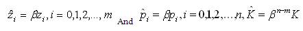
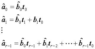
If, x(t) is a signal, w(t) = x(βt) is a time scaled version of x (t) and is speeded up if β > 1, and slowed down, if 0 < β < 1. Let, y(t) denote the forced response, to a step r(t), of a system with transfer function G(s). The authors are interested in determining a system with transfer function, H(s) so that, its forced response to r(t) is y(βt) for a given β > 0. H(s) speeds up the step response of G(s) by a factor β, [1]-[3]. Let,


Given G(s) as before, H(s) which speeds up the step response of G(s) by a factor β, is uniquely determined by one of the following equivalent conditions [1], [3]-[5]:
Proof:
Introducing the characteristic ratios and generalized time constant for a Hurwitz polynomial [1]-[3]:
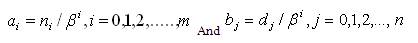
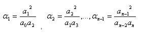
Characteristic ratios is given by,
and the generalized time constant is given by,

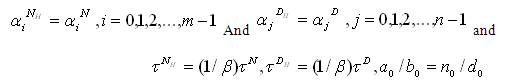
If G(s) is stable and minimum phase, then ni, di > 0 for all i’s without loss of generality, and the characteristic ratios of N(s) and D(s) are defined accordingly. Let the characteristic ratios of N(s), D(s), NH(s), and DH(s) be αiN, αiD,&al pha;iNH and αiDH respectively. Similarly, let the generalized time constants of those polynomials be, τN, τD, τNH and τDH , respectively.
If G(S) is stable and minimum phase, H(s) is uniquely determined by,
Remarks:
1) Equation (3) shows how the coefficients of H(s) can be obtained by scaling the corresponding coefficients of G(s).
2) Equation (4) shows that the poles and zeros of G(s) are moved out along rays from the origin by a factor of β, while the “DC” gain G(0) = H(0).
3) Equation (8) shows that the characteristic ratios of the numerators and denominators of H(s) remain unchanged, respectively, from those of G(s), while the generalized time constant of both numerator and denominator are reduced by a factor β.
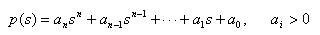
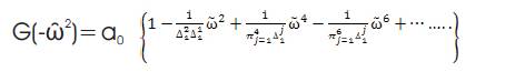
Let G(s) be an all-pole transfer function [1]-[5]:
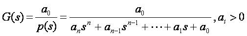
and let αi be the characteristic ratios of p(s). Then,
1) The frequency magnitude function |G(jω)| is monotonically decreasing and
2) p(s) is Hurwitz; if the following two conditions hold:
Proof:
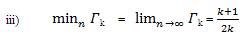
The detailed proofs can be found in [1]. To prove Theorem 2, the following lemma are necessary in describing the properties of Γk .
Lemma 1: For the definition of Γk in equation (7), we have the following
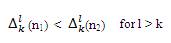
ii) Consider two polynomials of degrees n1 and n2 (n1 >n2 ) satisfying the equations (3) and (4) of Theorem 2 and let Γk (n1) and Γk(n2) be the corresponding Γk at n=n1and, n=n2 respectively. Then,
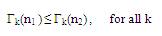
and equality holds at k=1.
Proof of Result-1:
Consider the square of frequency magnitude of a stable all-pole transfer function,
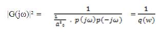
Using the relationships given in equations (2) and (3), q(w) is given in terms of the characteristic ratios αi and generalized i time constant τ of p(s).

Then,
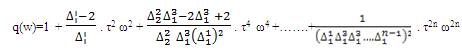
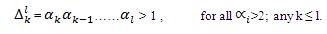
Result-1 is proved by showing that, the even degree function in equation (16) is a monotonically increasing function. The function q(w) is monotonically increasing if all j the coefficients are positive. Thus, all 's Δij are positive, q(w) is a monotonically increasing function if,
The proof is completed by showing that, equation (17) holds under the conditions of equations (3) and (4) in Theorem 2. It is not difficult to show by using lemma 1 that for k=1,2,3,…………, n-1,
This concludes the proof of the result (1) in Theorem 2.
Proof of Result-2:
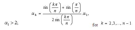
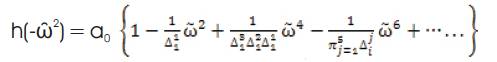
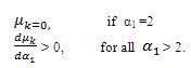
Note that p(s) is Hurwitz for α1 =2. Consequently, the nth order 1 polynomial image p(jω) |α1 =2 obeys the monotonic 1 phase increase the property and turns nπ/2 over ω∈ (0,∞) by the Mikhailov criterion [3]. Thus, it is enough to show that the phase of p(jω) is monotonically increasing over ω∈ (0,∞), for all α1 > 2. From equations (11), (12),and (15), with  ,
,
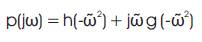
where,
Define
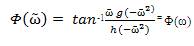
The monotonic phase increase property [3] of p(s), 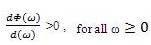 is equivalent to,

Rewriting equation (23), we have for n odd (i.e., n=2m+1)

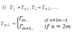
where for k=1, 2, 3,……,n-2. equation (26), shown below, holds. From the expression for the denominator of each term in equation (24), the phase monotonicity equation (23) is satisfied if all µI's in equation (25) are positive. From property, i) in Lemma 1,
µ1=µn-2 , =µn- 3.....................
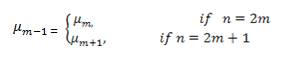
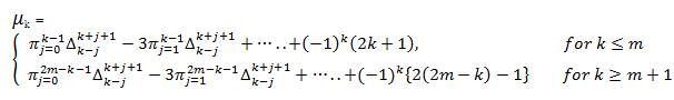
Therefore, it is enough to show that µ1 > 0 for I = 1,2,…., m or m-1. From property ii) in lemma 1, we also observe that the following is true.
where,
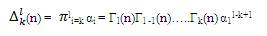
Under the condition in equation (26) ,it is clear that if, µi(ni) for all I are positive, µi(n) for all i are also positive for any such a i polynomial of degree n < ni . Thus, the proof of the result (2) is accomplished by showing that, µi(n) for all i are positive when,n→∞.
It can be shown by using equation (26) and (28) that for k = 1,2,3,…..,n-2,
Thus the proof is completed.
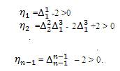
The authors establish this theorem by showing that, all ηi ≥ 0 when all αi > 2. Recall equation (17) and write,
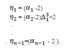
Observe that,
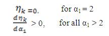
Thus, for α1 > 2, I =1,2,3,….,n-1, every ηkis positive.
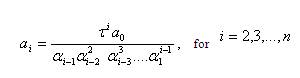
The coefficients of p(s) is calculated from characteristic ratios and time constant, as follows:

Let us consider three all pole transfer functions, Tk (s) = a0 /Pk(s) of different orders, but having the same α1 and α2 , which are chosen to obtain sufficiently large α 1x α2 . All parameters and coefficients are shown in Table 1, and the step responses of these transfer functions are shown in Figure 1. Therefore the theorem is proved.
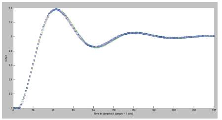
Figure 1. Step Response Comparison (Table 1)
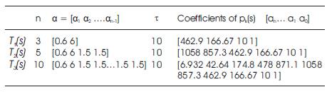
Table 1. Parameters of Three Transfer Functions
Even though the three transfer function models are quite different, except having similar values of α1 , α2 and τ; surprisingly, they have almost the same step responses. This result is caused by the dominance of the characteristic ratios α1 and α2 . This idea helps in reducing the order of the denominator of a transfer function that has dominant characteristic ratios α1 and α2 .
Remarks
1) The authors experience also shows that increasing α1 reduces overshoot.
2) Reducing order of the denominator of transfer function which is having dominant characteristic ratios α1 and α2 .
This idea of characteristic ratio assignment can be used to reduce the order of the denominator of a higher-order of all pole transfer function. Now, the focus will be to find methods to reduce the order of numerator of a general transfer function so that, the step response of the reduced transfer function matches the original system as closely as possible.
To reduce the order of numerator, the authors have considered four methods, of which first three methods use the CRA technique to find the Reduced Order Denominator (ROD). The methods are [5], [6], [8]-[10]:
1. Time moment matching.
2. Time moment and Markov parameter matching.
3. Approximate Generalized Time Moment (AGTM) matching.
4. AGTM matching for obtaining the complete Reduced Order Model (ROM).
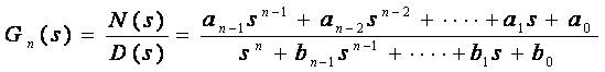
Consider a SISO system described by a transfer function of order 'n'.
The problem is to determine its stable reduced-order (rth - order) approximate:
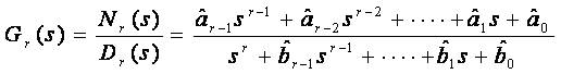
Gn(s) is a given transfer function and Dr(s) is found by obtaining reduced order denominator D(s) of the original transfer function G(s) through the CRA technique. The order 'r' of Dr(s) is the minimum 'r' value up to which the step r response of transfer function (1/Dr(s)) tracks the step response of transfer function (1/D(s)) as closely as possible.
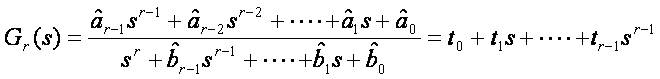
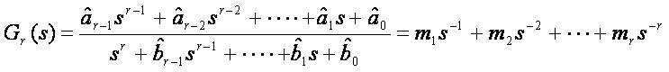
Expanding Gn(s) around s = 0:

To find the reduced numerator, equate Gr(s) to the above expansion:
Multiplying the above equation with Dr(s) (known from CRA) on both sides, and equating the coefficients of equal power of 's'; after simplification, the reduced numerator coefficients are obtained by solving the following equations:
The numerator coefficients of the reduced model obtained by this method ensures good low frequency (large time) matching i.e., steady state matching of the original system and reduced order model because the expansion of Gn(s) has been done around s=0.
Expanding Gn(s) around s = ∞, one obtains:

Equating Gr(s) to the above expansion, the reduced r numerator polynomial can be obtained. Thus,
Multiplying the above equation with Dr(s) (known from CRA) on both sides, and equating the coefficients of equal powers of 's'; after simplification, the reduced numerator coefficients are obtained by solving the following equations:
The numerator coefficients of the reduced model obtained by this method ensures good high frequency (transient state) matching of the original and reduced transfer functions because expansion of Gn(s) is taken around s=∞.
Now, we know the reduced numerator from both complete time moment matching and complete Markov parameter matching. In order to obtain a good overall matching of time responses of Gr(s) to Gn(s) in both transient and steady states, one should match α time moments and β Markov parameters, so that α + β = r, the number of unknown parameters in the numerator polynomial. The best values of α and β to be chosen, depends on the system to be reduced, and cannot be determined a-priori. This is an open problem for further research.
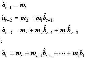
In this method, we will equate the Gr(s) and Gn (s) at specific real values of 's'.
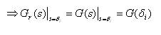
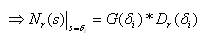
where, δ=0.01 and δi=δ*i, for i =1,2,…,r for steady state matching; like time moment matching, and δi=(1/δ)*i, for i =1,2,…,r for transient state matching like Markov parameter matching.

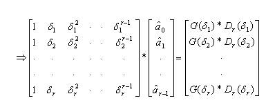
This is in the form of A.x=B and the reduced numerator coefficients can be easily obtained by solving the set of appropriate linear algebraic equations. One should choose an appropriate combination of δi=δ*i and/or δi=(1/δ)*i values so that, total number of δi values = 'r'; thus ensuring a good overall time response approximation.
It is similar to the above method, but here both the numerator and denominator of reduced transfer function are taken as unknowns. So here we should choose total 2r number of δi values to find 'r' number of reduced denominator coefficients and 'r' number of reduced numerator coefficients. Proceeding as above and bringing the known terms to one side, and the unknown terms to other side, and on rearranging, the equation in matrix form will be obtained as below:

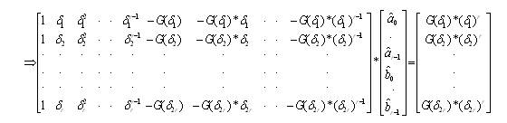
The matrix solution of a set of linear algebraic equations are applied to the above matrix equation and the numerator and denominator coefficients of the ROM are obtained.
In the following, the authors have consider several examples from the literature for order reduction by using all the above four methods. The results will be compared to find the best reduction method. For comparison, a performance index is chosen as the sum of square of error in step responses of G(s) and Gr(s) at the chosen sampled points. Let Y(t) and Yr(t) are the step responses of G(s) and Gr(s). Then the performance index is taken as:
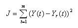
where, m is the number of sampled points.
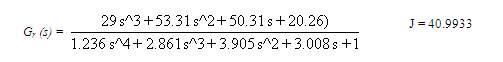
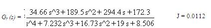
The given high order transfer function is taken from [7] where,
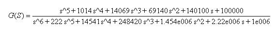
Reduced order transfer functions are obtained as:
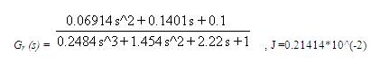
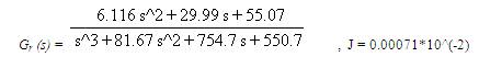
1. Complete time moment matching gives:
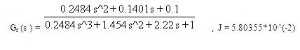
2. Two Time moment and One Markov parameter matching gives:
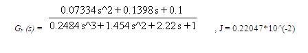
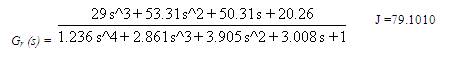
3. AGTM matching for obtaining the numerator polynomial gives:
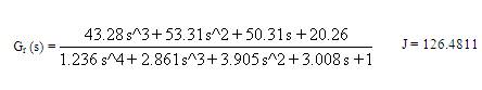
4. AGTM matching for obtaining the ROM gives:
In Figure 2, the step responses of the above transfer functions for example 1 are shown.
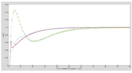
Figure 2. Step Response Comparison (Example 1)
The following high order plant transfer function is taken from [14] where,

The calculated reduced order transfer functions are:
1. Complete time moment matching gives:
2. By matching three time moments and one Markov parameter:
3. AGTM matching for numerator only gives:
4. AGTM matching for both the numerator and denominator gives:
In Figure 3, the step responses of the above transfer functions for Example 2, are shown.
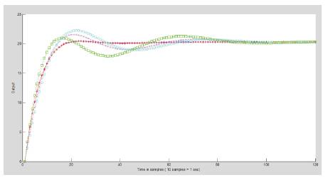
Figure 3. Step Response Comparisons (Example 2)
From Figures 2 and 3, the ROMs obtained by different methods, one can conclude that the AGTM method for obtaining ROM gives the best result in matching the original transfer function response.
Various methods are described to reduce the order of higher-order continuous time, SISO or MIMO transfer. The methods are illustrated by solving several examples froms the literature. In the reduced order modeling method using “time moment and Markov parameter matching”, the number of time moments and Markov parameters to be matched, and the optimal combination to be chosen is open to further investigation.