The operation of an electric power system is a complex one due to its nonlinear and computational difficulties. One task of operating a power system economically and securely is optimal scheduling, commonly referred to as the Optimal Power Flow (OPF) problem. It optimizes a certain objective function while satisfying a set of physical and operating constraints. Optimal power flow has become an essential tool in power system planning and operation. In this paper, a gravitational search algorithm is presented to solve OPF problems while satisfying system equality, in-equality constraints. The effect of security limits such as transmission line limits and load bus voltage magnitudes is also analyzed on OPF problem. The developed methodology is tested on the standard IEEE-30 bus test system, supporting numerical as well as graphical results.
For secure operation of the system without any limit violation, complete modeling of the system through load flow equations and operational constraints is necessary. Thus the Optimal Power Flow (OPF) is a good choice. The solution of formulated Optimal Power Flow (OPF) model gives the optimal operating state of a power system and the corresponding settings of control variables for economic and secure operation, while at the same time satisfying various equality and inequality constraints. The equality constraints are the power flow equations, while the inequality constraints are the limits on control variables and the operating limits of power system dependent variables. Amongst a number of different operational objectives that an OPF problem may be formulated, a widely considered objective is to minimize the fuel cost subject to equality and inequality constraints.
The goal of optimal power flow is to determine optimal control variables and quantities for efficient power system planning and operation. Several optimization techniques have been proposed to handle the OPF problem [1-3]. A wide variety of optimization techniques have been applied to solve the OPF problems such as Nonlinear Programming (NLP) [1, 4-10, 11-13], Quadratic Programming (QP) [6,7], Linear Programming (LP) [14, 15], Newton-based techniques [8, 9], and sequential unconstrained minimization technique [10]. Generally, NLP based procedures have many drawbacks such as insecure convergence properties and algorithmic complexity.
Another evolutionary computation technique called Particle Swarm Optimization (PSO), has been proposed and introduced [16-19]. This technique combines social psychological principles in socio-cognition human agents and evolutionary computations. PSO has been motivated by the behavior of organisms such as fish schooling and bird flocking. Generally, PSO is characterized as simple in concept, easy to implement and computationally efficient. Unlike, the other heuristic techniques, PSO has a flexible and well-balanced mechanism to enhance and adapt to the global and local exploration abilities.
In this paper, the PSO and GSA (Gravitational Search Algorithm) based algorithms for solving OPF problems, with generation fuel cost as objective, is presented. The effect of security constraints on OPF problem is investigated by considering security limits. The proposed approach has been tested on the Standard IEEE-30 bus system. The potential and effectiveness of the proposed approach are demonstrated.
The aim of the Optimal Power Flow solution is to optimize the selective objective function through proper adjustment of control variables by satisfying various constraints. The OPF problem can be represented as follows:

Subjected to g(x,u) = 0 and
hmin≤h(x,u) ≤hmax
where,
Am (x,u) is the function which is to be minimized,
g(x,u), h(x,u) represents equality and inequality constraints, ‘x' and 'u' are dependent and independent variables.
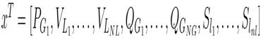
Optimal power flow solution gives an optimal control variable leads to the minimum generation fuel cost, emission and total power loss, etc. subjected to all the various equality and inequality constraints. Here, the vector 'x' consists of slack bus real power output (PG1 ), generator VAr output (QG ), load bus voltage magnitude (VL ), and line flow limits (SI ).
Thus 'x' can be written as,
where,
NL = Number of load buses,
NG = Number of generator buses,
nl = Number of lines,
u = the independent variable vector such as continuous and discrete variables that consists of,
Here PG , VG are continuous variables and T and QC are the discrete variables. Hence 'u' can be expressed as,
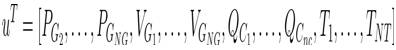
'NT' and 'nc' are the number of tap controlling transformers and shunt compensators.
The main aim of OPF problem is to optimize the total generation fuel cost in a system. Generators for which fuel cost characteristics are given by,
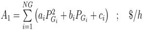
where, ai , bi , ci are the fuel cost coefficients of ith unit. PG! is the active power generation of ith unit.
Constraints made in this OPF problem are usually two types. They are equality constraints and inequality constraints.
These constraints mentioned in Equation (2) are usually load flow equations described as,
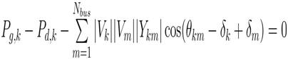
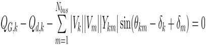
where, PG,K , QG,K are the active and reactive power generation at the kth bus, Pdk , Qdk are the active and reactive power demands at the kth bus, |Vk| | Vm| are the voltage magnitudes at the kth and mth buses, δk , δm are the phase angles of the voltage at the kth and mth buses, and |Ykm| , θkm are the bus admittance magnitude and its angle between the kth and mth buses.
These are the constraints that represents the system operation and security limits which are continuous and discrete constraints.
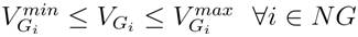
Generator bus voltage limits:
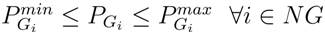
Active power generation limits:
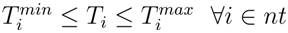
Transformers tap setting limits:
Capacitor reactive power generation limits:
Transmission line flow limit:
Reactive power generation limits:
Load bus voltage magnitude limits:
The control variables in this problem are self-constrained, whereas the in-equality constraints such as PGi , VI , QGi , and Sli are non-self-constrained by nature. Hence, these inequalities are incorporated into the objective function using a penalty approach [8]. The augmented function can be formulated as:
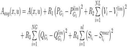
where, R1 , R2 , R3 and R4 are the penalty quotients, which take large positive values. The limit values of the dependent variable xlim can be given as:
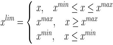
where, xlim can be PG1 , Vi , QGi
Particle Swarm Optimization (PSO) is a population based stochastic optimization technique developed by Dr. Eberhart and Dr. Kennedy in 1995, inspired by social behavior of bird flocking or fish schooling [20].
PSO shares many similarities with evolutionary computation techniques such as Genetic Algorithms (GA). The system is initialized with a population of random solutions and searches for optima by updating generations. However, unlike GA, PSO has no evolution operators such as crossover and mutation. In PSO, the potential solutions, called particles, fly through the problem space by following the current optimum particles.
PSO has been successfully applied in many research and application areas. It is demonstrated that, PSO gives better results in a faster, cheaper way compared with other methods [21].
PSO is initialized with a group of random particles (solutions) and then searches for optima by updating generations, the particles are "flown" through the problem space by following the current optimum particles. Each particle keeps track of its coordinates in the problem space, which are associated with the best solution (fitness) that it has achieved so far. This implies that each particle has a memory, which allows it to remember the best position on the feasible search space that it has ever visited. This value is commonly called pbest . Another best value that is tracked by the particle swarm optimizer is the best value obtained so far by any particle in the neighborhood of the particle. This location is commonly called gbest . The basic concept behind the PSO technique consists of changing the velocity (or accelerating) of each particle toward it's pbest and the gbest positions at each time step. This means that each particle tries to modify its current position and velocity according to the distance between its current position and pbest , and the distance between its current position and gbest .
PSO, simulation of bird flocking in two-dimension space can be explained as follows. The position of each agent is represented by XY-axis position and the velocity is expressed by VX (the velocity of X-axis) and VY (the velocity of Y-axis). Modification of the agent position is realized by the position and velocity information. PSO procedures based on the above concept can be described as follows. Bird flocking optimizes a certain objective function. Each agent knows its best value so far (pbest ) and its XY position. Moreover, each agent knows the best value in the group (gbest ) among pbest . Each agent tries to modify its position using the current velocity and the distance from pbest and gbest . The modification can be represented by the concept of velocity. The new velocity and updated positions are calculated using the following expressions,
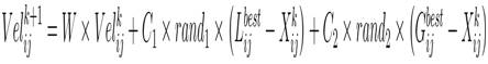
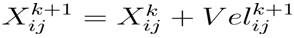
where, 'Xijk ' and 'Velijk ' are the present position and velocities of ith particle in jth dimension in kth iteration. These new velocities and updated positions are calculated repeatedly for a pre- defined number of iterations reached. For minimization of the objective functions, the fitness function is evaluated using the following expression,
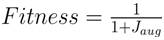
Expressions (16) and (17) describe the velocity and position update, respectively. Expression (16) calculates a new velocity for each particle based on the particle's previous velocity, the particle's location at which the best fitness has been achieved so far, and the population global location at which the best fitness has been achieved so far. Usually C1 =C2 =2.
The complete procedure of PSO is shown in Figure 1.
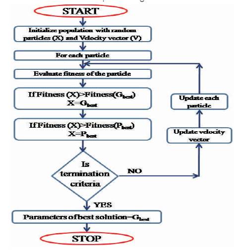
Figure 1. Flow Chart of Existing PSO
In this section, the developed algorithm is based on the law of gravity. In the proposed algorithm, agents are considered as objects and their performance is measured by their masses. All these objects attract each other by the gravity force, and this force causes a global movement of all objects towards the objects with heavier masses. Hence, masses co-operate using a direct form of communication, through gravitational force. The heavy masses – which correspond to good solutions – move more slowly than lighter ones, this guarantees the exploitation step of the algorithm.
In GSA, each mass (agent) has four specifications: position, inertial mass, active gravitational mass, and passive gravitational mass. The position of the mass corresponds to a solution of the problem, and its gravitational and inertial masses are determined by using a fitness function.
In other words, each mass presents a solution, and the algorithm is navigated by properly adjusting the gravitational and inertia masses. By lapse of time, we expect that the masses be attracted by the heaviest mass. This mass will present an optimum solution in the search space.
The GSA could be considered as an isolated system of masses. It is like a small artificial world of masses obeying the Newtonian laws of gravitation and motion. More precisely, masses obey the following laws:
Each particle attracts every other particle and the gravitational force between two particles is directly proportional to the product of their masses and inversely proportional to the distance between them, R. The authors use R instead of R2 because according to the experiment results, R provides better results than R2 in all experimental cases.
The current velocity of any mass is equal to the sum of the fraction of its previous velocity and the variation in the velocity. Variation in the velocity or acceleration of any mass is equal to the force acted on the system divided by mass of inertia.
The gravitational constant, G, is initialized at the beginning and will be reduced with time to control the search accuracy. In other words, G is a function of the initial value (G0 ) and time (t):
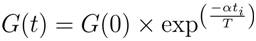
where, α is a constant, ti is the iteration number and 'T' is the total number of iterations.
Consider a system of N agents. The position of ith agent is defined as,
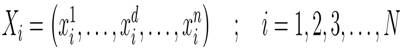
For each position, fitness function is evaluated.
Let, fit i(t) be the fitness function of ith particle at tth iteration.
Now, the authors introduce new variables worst (t) and best (t).
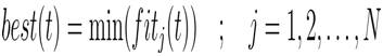
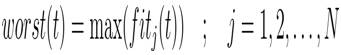
For a minimization problem, best (t) and worst (t) are defined as follows:
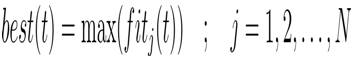
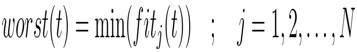
For a maximization problem, best (t) and worst (t) are defined as follows:
Gravitational and inertia masses are simply calculated by the fitness evaluation. A heavier mass means a more efficient agent. This means that, better agents have higher attractions and walk more slowly. Assuming, the equality of the gravitational and inertia mass, the values of masses are calculated using the map of fitness. The gravitational and inertial masses are updated by the following equations:
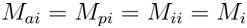
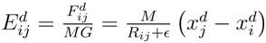
For iteration t, the force acting on mass i from mass j is defined as the following,
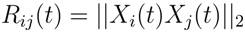
where, Maj , Mpi are the active and passive gravitational masses related to agent j, G(t) is gravitational constant at iteration t, ε is a small constant and Rij is the Euclidian distance between two agents i and j given by,
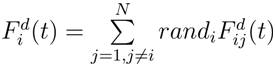
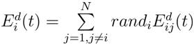
To give a stochastic characteristic to the algorithm, the total force that acts on agent i in a dimension dth be a randomly weighted sum of d components of the forces exerted from other agents:
One way to perform a good compromise between exploration and exploitation is to reduce the number of agents with lapse of time. Hence, the authors propose only a set of agents with bigger mass apply their force to the other. However, we should be careful of using this policy because it may reduce the exploration power and increase the exploitation capability.
The authors remind that, in order to avoid trapping in a local optimum, the algorithm must use the exploration at beginning. By lapse of iterations, exploration must fade out and exploitation must fade in. To improve the performance of GSA by controlling exploration and exploitation only the Kbest agents will attract the others. Kbest is a function of time, with the initial value K0 at the beginning and decreasing with time. In such a way, at the beginning, all agents apply the force, and as time passes, Kbest is decreased linearly and at the end there will be just one agent applying force to the others.
Therefore, equation (30) can be modified as:
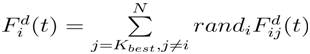
where, Kbest is the set of first K agents with the best fitness value and biggest mass given by,
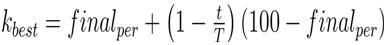
where, finalper is the percentage of particles that remain at the end (generally 2). Since M is a function of m, which is function fitness, in every iteration, one value of m is zero. Hence, M is zero at this value of m. At this value of M, acceleration becomes an indefinite value from above equations. To obtain integer value of Kbest , it is rounded in terms of population. Hence, we introduce another variable E which is defined as follows:
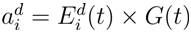
Hence, by the law of motion, the acceleration of the agent 'i' at iteration t , and in direction d, is given as:
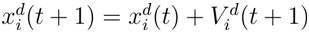
Furthermore, the next velocity of an agent is considered as a fraction of its current velocity added to its acceleration. Therefore, its position and its velocity could be calculated as follows:

The different steps of the proposed algorithm are following.
The complete procedure of GSA is shown in Figure 2.
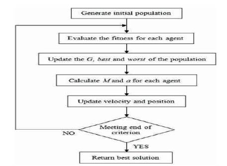
Figure 2. Flow Chart of GSA
In order to demonstrate the effectiveness and robustness of the proposed GSA method, the Standard IEEE 30 bus system is considered. The existing and proposed methodologies are implemented on a personal computer with Intel Core2Duo 1.18 GHz processor and 2 GB RAM. The input parameters of the existing PSO method and the proposed GSA method for the considered test system are given in Table 1.

Table 1. Input Parameters for Test System
This section presents the details of the study carried out on the Standard IEEE-30 bus test system to analyze OPF problem. The network and load data for this system is taken from [1]. In the Standard IEEE-30 bus system consist of 41 branches, six generator buses and 21 load buses. Four branches 6-9, 6-10, 4-12 and 27-28 have tap changing transformers. The buses with possible reactive power source installations are 10 and 24.
The effectiveness of SCOPF (Security Constrained Optimal Power Flow) over OPF is verified using existing PSO and proposed GSA. The respective results are tabulated in Table 2. From this table, it is observed that, less generation fuel cost is obtained with the proposed GSA when compared to the existing PSO algorithm in OPF and SCOPF problems.
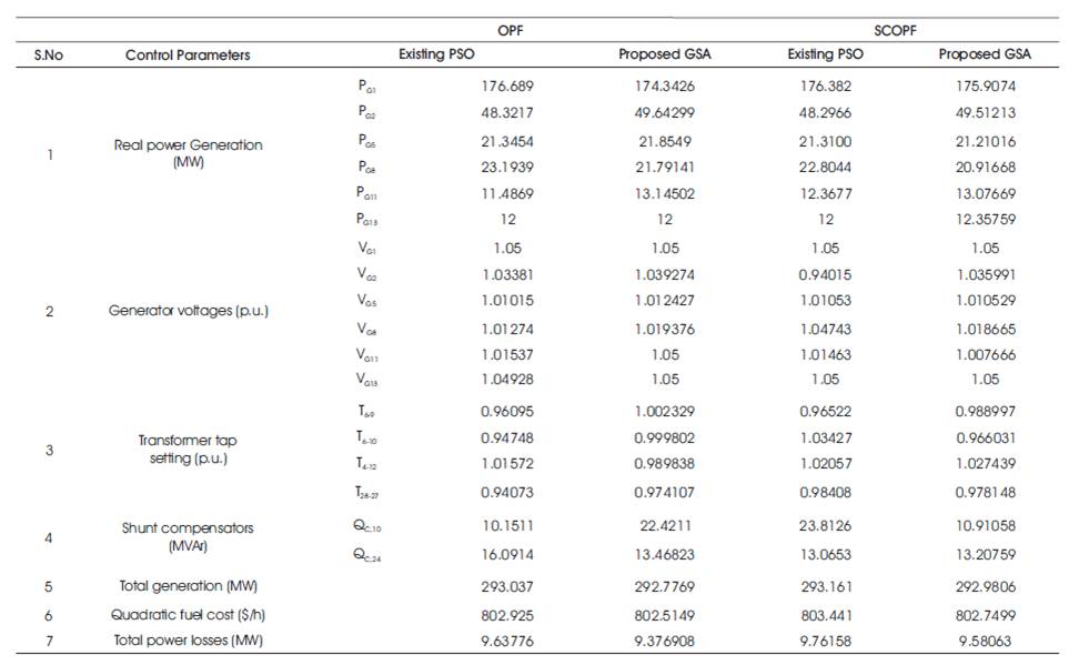
Table 2. OPF and SCOPF Results of Generation Fuel Cost for Standard IEEE-30 Bus System
Using the proposed GSA, the total generation and there by the total transmission power losses are decreased. It is also observed that, because of the increased number of constraints in SCOPF, the generation fuel cost is increased when compared to OPF. In OPF problem, using the proposed GSA, the generation fuel cost in decreased by 0.4107 $/h and whereas in SCOPF problem, the generation fuel cost is decreased by 0.6916 $/h.
The convergence characteristics for the OPF and SCOPF problems using the existing and proposed methods are shown in Figures 3 and 4. From these Figures 3 and 4, it is observed that, in both of the problems, the proposed GSA algorithm starts the iterative process with better initial value and converges to a best value in less number of iterations when compared to the existing PSO algorithm. It is also identified that, because of the increased number of constraints in SCOPF problem, the convergence starts with higher generation fuel cost value when compared to that of OPF problem.
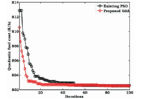
Figure 3. Convergence Characteristics of OPF with Quadratic Cost for IEEE-30 Bus System
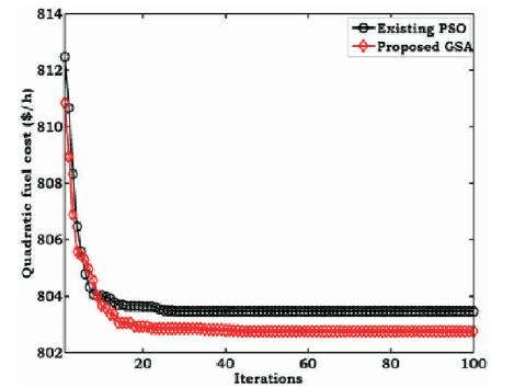
Figure 4. Convergence Characteristics of SCOPF with Quadratic Cost for IEEE-30 Bus System
The voltage magnitudes at buses in OPF and SCOPF problems are tabulated in Table 3. Similarly, the variation of voltage magnitudes in OPF and SCOPF problems using the existing and proposed methods is shown in Figures 5 and 6. From Figure 5, it is observed that, because of solving OPF problem without security limits, voltage magnitude deviations are high at some of buses and majority of buses are operating nearer to maximum voltage limit. From Figure 6, it is observed that, because of SCOPF problem, the voltage magnitude at buses is within its voltage limits. It is also observed that, in both of the problems, with the proposed GSA, the voltage magnitude at buses is enhanced when compared to the existing PSO algorithm.
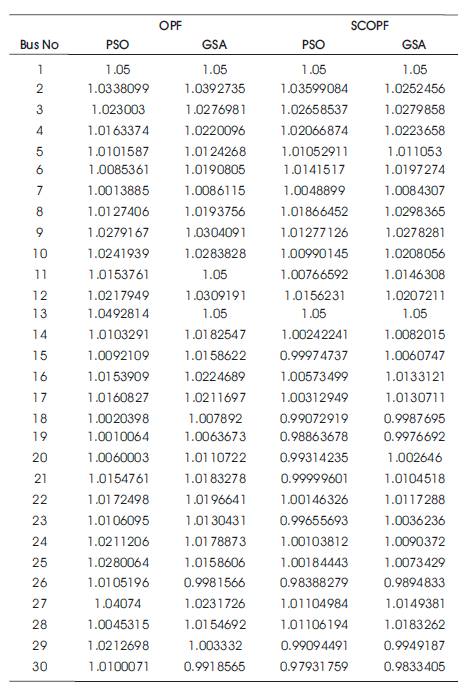
Table 3. Voltage Magnitudes of OPF and SCOPF with Quadratic Cost for IEEE-30 Bus System
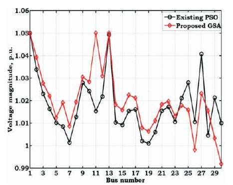
Figure 5. Variation of Voltage Magnitudes of OPF with Quadratic Cost for IEEE-30 Bus System
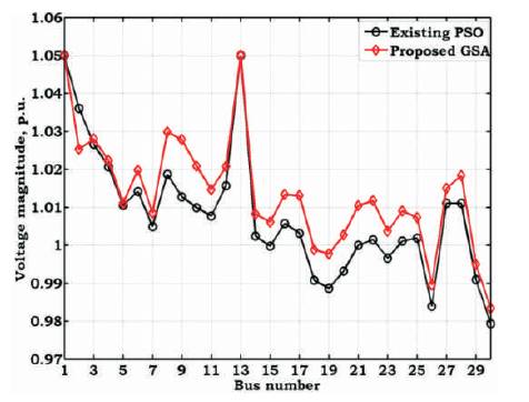
Figure 6. Variation of Voltage Magnitudes of SCOPF with Quadratic Cost for IEEE-30 Bus System
Similarly, the transmission line power flows in OPF and SCOPF problems using existing and proposed methods are tabulated in Table 4 and the respective variation is shown in Figures 7 and 8. From Figure 7, it is observed that, because of solving OPF problem without security constraints, the power flow in some of the lines is operating nearer to the maximum MVA limit. From Figure 8, it is observed that, because of SCOPF, the power flow in all lines is within limits. In this problem, the power flow in some of the lines is reduced with the proposed GSA when compared to the existing algorithm.
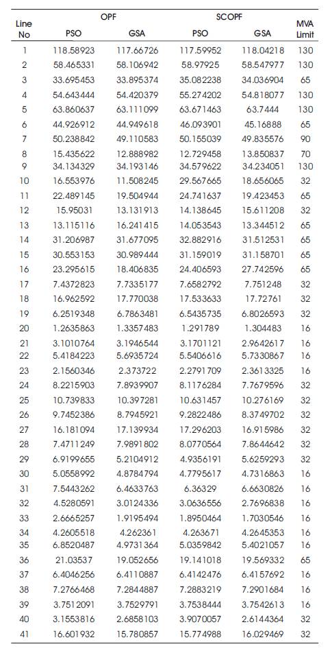
Table 4. Power Flows of OPF and SCOPF with Quadratic Cost for IEEE-30 Bus System
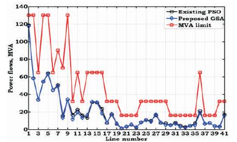
Figure 7. Variation of Power Flows of OPF with Quadratic Cost for IEEE-30 Bus System
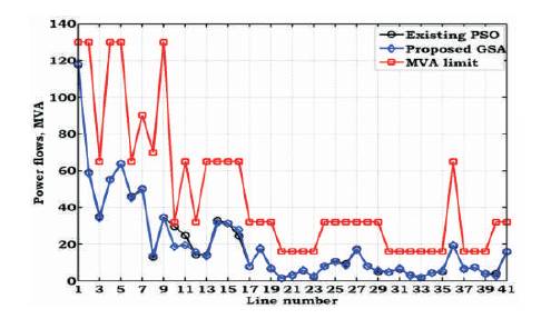
Figure 8. Variation of Power Flows of SCOPF with Quadratic Cost for IEEE-30 Bus System
To support the effectiveness of the proposed method, obtained results are compared with the existing literature methods. The comparison results is given in Table 5. From this table, it is identified that, the proposed method yields good results when compared to the existing methods
From the above analysis, it has been concluded that, because of including security constraints in SCOPF problem, this problem is more efficient when compared to OPF problem. From this, it is assumed that, further analysis is performed using SCOPF only.
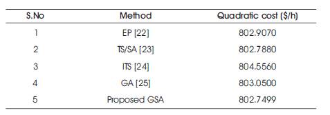
Table 5. Validation of SCOPF results of quadratic cost for IEEE-30 bus system
In this paper, to show the effect of security constraints on OPF problem which has been demonstrated by performing OPF and SCOPF problems by considering generation fuel cost as objective. To solve this problem, Gravitational Search Algorithm (GSA) is proposed. The effectiveness of the proposed algorithm is compared with the existing Particle Swarm Optimization (PSO). The effect of security constraints on voltage magnitudes and line power flows has been analyzed. The complete methodology has been tested on the standard IEEE-30 bus test system. The obtained results are validated with the existing literature.