Big Data corresponds to the huge volume of data. In the recent years, big data is becoming a crucial area of research. Big data are used in marketing sectors, banking sectors, medical systems, etc., for its immense use. In order to retrieve useful information from the huge volume of data, datamining methods are employed. The underlying concept in the datamining process is feature selection.

Feature selection refers to extraction of similar kinds of elements or particles or data. It is one of the critical step for various reasons[4]. Feature selection involves in the selection of predetermined number of features which leads to the performance enhancement of the total classifier. This technique is employed in various fields such as in text classification, speech recognition and medical diagnosis. But practically, there is a need to reduce the number of measurements without degrading the performance of the system[3].

The risk or complexity is high in feature selection because of complex interaction between the features. Another factor, i.e size of the search space is directly proportional to increase in complexity of feature selection process. The size increases in an exponential manner based on the number of features present in the dataset. There are different kinds of methods employed in the feature selection process with various dimension measures[2]. In the recent years, many strategies have come into foray to obtain optimal solutions for different problems, Evolutionary algorithms such as ant colony algorithm, genetic algorithm and Particle swarm optimization algorithm are used in optimization techniques.

Feature Selection algorithms have the capabilities to improve the performance in the classification process [10].

1.1 Genetic Algorithms

In the Genetic Algorithms, a group of particles or a swarm of particle or candidate solutions is evolved in an optimization for obtaining better solution. Genetic algorithms are independent and can be applied to various problems irrespective of the domain area. Over the years Genetic Algorithms have made a substantial improvement in the random as well as local search techniques, which also called as adaptive search techniques. The algorithm proceeds by collecting information about its neighborhood particles and forwards till it finds the best solution to the given search space[7]. One of the main disadvantages arousing in genetic algorithms for feature selection is the selection of evaluating function or fitness function. The efficiency and performance of the system depends upon the objective function which is chosen to evaluate the system. It forms the basis for the performance analysis.

1.2 Particle Swarm Optimization

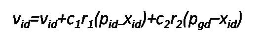
Particle Swarm Optimization was first developed by Eberhart and Kennedy in 1995[1] with a view of simulation of social system. This method has been tremendously utilized in various applications. Particle Swarm Optimization is an evolutionary computing technique. One of the major difference between evolutionary computing technique and Particle Swarm Optimization is, the former one uses genetic operators and the latter one uses physical movements of individuals in the swarm. One of the most beguiling features that provoke us to use PSO is its simple procedure and few parameters. PSO is similar to Genetic algorithm, for example it starts with neighborhood with randomly generated swarm, calculation of fitness value, evaluating, later updating of the position and search for the optimal solution, but it could not ensure the optimal solution. It consist of two best fit or best value. They are called Pbest and Gbest. Pbest corresponds to the best value that has been obtained so far and the Gbest corresponds to the best value it has achieved in the global space or the population. Pbest is also called local optimal solution and Gbest is called global optimal solution. The particle in the swarm are represented in N-Dimensional space and are characterized by their position and velocity[8]. The original or standard PSO is given as ,

(1)

(2)

The modified PSO[6] equation is given below.

(3)

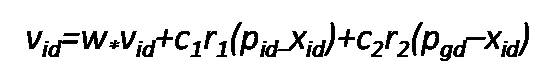
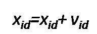
In the above equation, d represents the set of natural numbers ranging from {1…..n}and i represents the index from 1 to S. S is the size of the population (i.e, swarm). The inertia weight factor w is used in the modified PSO. The c₁ and c₂ are constants which are known as cognitive and  social components, also the acceleration parameters and r₁ , r₂ are the random numbers. v_id is the velocity vector and X_id is the position vector. The PSO algorithm is used in  several applications such as scheduling process[9], feature selection, optimization, etc.

1.3 Fast Feature Selection Algorithm

Feature selection techniques which are previously discussed have their own advantages and disadvantages. Some have the capability to remove redundant data and some have the capability to remove irrelevant data. For example Chi square algorithm has the capability to remove irrelevant data [5]. In order to balance the both the authors have used FAST algorithm. This FAST feature selection technique has the capability to reduce both the anomalies in a balanced way.

1.4 Motivation

Feature Selection has been a key interest in recent years because of its wide uses and applications. It is pursued with great interest because of some of the following problems.

• In Datamining applications such as classification.
• Need for extraction of relevant and accurate features to analyze the huge data.
• When different parameters are merged, there is a need to integrate different such models.

2.1 Algorithm

Feature subset.

Inputs: D (F₁ ,F₂ ,….,F_m ,C) the given dataset

ϴ-the T-Relevance threshold.

Output: S- selected

//Irrelevant Feature removal

for i-1 to m do

T-Relevance = SU (F_i ,C)

If T-Relevance> ϴ then

S=S U({F_i };

//Minimum Spanning Tree Construction

G=NULL; //G is a complete graph

for each pair of feature {F_i ',F_j '} ⊂S do

F-Correlation- S U {F_i^i',F_j '}

Add F_i ' and /or F_j ' to G with Correlation as the weight of the  corresponding edge

minSpanTree-Kruskals (G); //using Kruskal Algorithm to generate the minimum spanning tree

//Tree Partition and Feature Subset Representation

Forest=minSpanTree

for each edge E_ij ∈ Forest do

if S U (F_i ',F_j ')< S U (F_i ,C) Ù S U (F_i ',F_j ')< S U (F_i ',C) then

Forest= Forest- E_ij

for each tree T_i ∈ Forest do

F_R'=argmax F_k∈T_i S U (F_k ',C)

S=

return S.

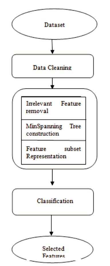
Figure 1. Data Flow Diagram of FAST Algorithm

2.2 Description

Fast algorithm is used in order to overcome the drawback and removes the irrelevant and redundant features. The Fast algorithm works in three phases, the first phase involves irrelevant feature removal, where the irrelevant feature is removed using the T- relevance. The second phase involves construction of minimum spanning tree, this process is useful in removing the redundant data present in the dataset. The third phase involves partitioning of tree and feature selection representation.

The foremost step involved in the experimental process is loading the data in the form of a dataset. Here, the authors have used the lung cancer dataset comprising of a set of attributes. During the loading process, preprocessing takes place, missing values and noisy data are removed by converting it in the ARFF (Attributed Related File Format) format.

After the conversion process, a table is created in the database, then the data is extracted from the database. Followed by extraction, the table is classified based on the last attribute. The classification is based on Naïve Bayes classification. Information gain is calculated in order to know the relevance of the attributes. Conditional entropy is calculated to know about the additional information about the attribute. The SU (Symmetric Uncertainty) is calculated by sharing the mutual gain information.

Hence entropy, conditional entropy and gain is calculated. In the next step, T-Relevance is calculated. During this process, irrelevant and redundant data are removed.

In the next phase, f-correlation is calculated. The strong correlation between the attributes signify those features that are more relevant. Minimum spanning tree is constructed using Kruskal's algorithm and unnecessary edges are eliminated. The Kruskal's algorithm follows a greedy approach. The unnecessary edges are removed where the edge value is less than that of the threshold value. This step is very much helpful in removing redundancy.

Standard deviation are calculated in order to find the information about the neighboring feature which have the high relevance which is given in Figures 2 and 3. Information gain and conditional entropy are calculated which is used to measure the mutual information between the features (shown in Figure 4).

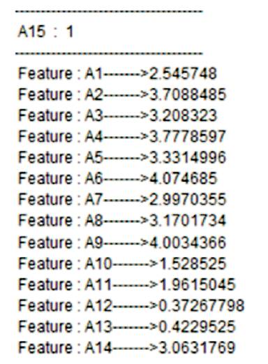
Figure 2. Standard Deviation Table for Class Label 1

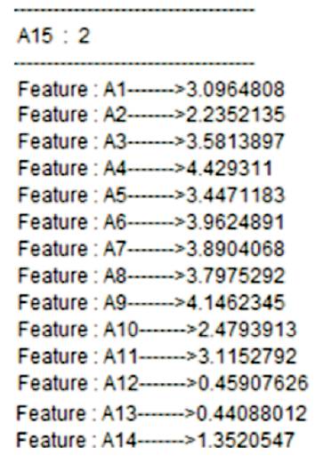
Figure 3. Standard Deviation for Class Label 2

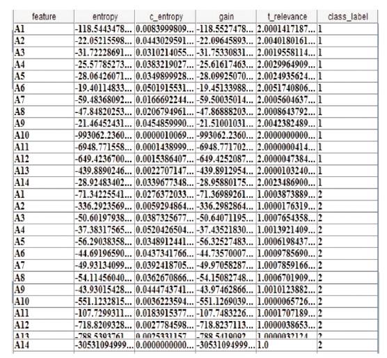
Figure 4. Entropy, Conditional Entropy, Gain and T- Relevance Calculation

3.1 Redundancy Removal

Redundant data are removed after the T-relevance calculation. The following attributes subset are obtained after the relevance calculation i.e., {A2, A3, A4, A5, A6, A9, A14} are obtained for class 1 label after redundancy removal and {A3, A4, A5, A6, A7, A8, A9} for class 2 label. Based upon these obtained attribute set, the F correlation is calculated. Figure 4 represents the F-Correlation values for the attributes of class label 1 and Figure 5 represents the F-Correlation values for the class label 2. The clusters are formed based upon their correlations.

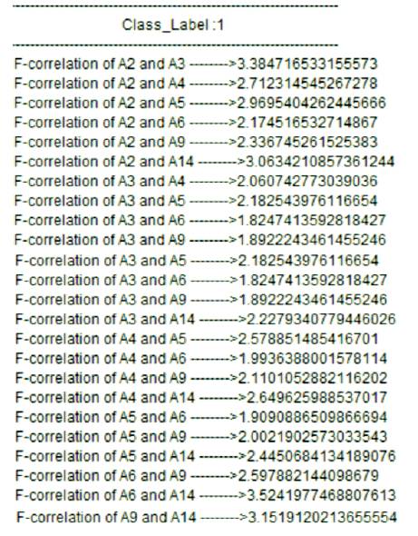
Figure 5. F-Correlation of Class Label 1

Correlations are generally used to know the linear relationship or monotonic relationship between two variables. As correlations are calculated between features, it is called F-Correlation which is shown in the Figure 5 and Figure 6. Uncertainty reduction is done through mutual information concept. Mutual information concept uses information gain concept in order to know the information content present in the concept. The main intent is to select only the required variables which account for more information, i.e “80-20” rule, where 20% of variable accounts for 80% of information.

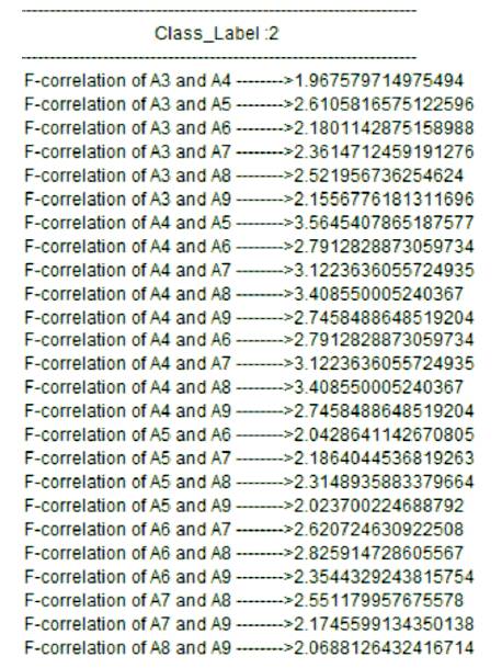
Figure 6. F-Correlation of Class Label 2

The same process is tested upon different datasets such as cancer, heart and lung cancer datasets. The obtained results are shown in the form of graphical representation for both Particle Swarm Optimization and FAST algorithms.

The graph in the Figure 7 shows the number of attributes selected vs Datasets. The FAST algorithm produces less number of attributes which are more effective than the PSO algorithm.

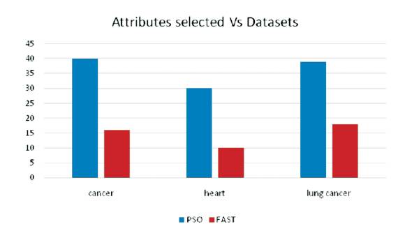
Figure 7. Comparison of Attributes Selected by PSO and FAST

In the present context, the authors have experimented the feature selection process using FAST feature selection algorithm. Although, there are several feature selection algorithms, the proposed feature selection algorithm has shown the positive results compared to the rest of the feature selection algorithms such PSO, Relief, Chi-square, etc. They found out that this technique more effectively selects the required effective attributes by avoiding redundant and irrelevant attributes. Hence, it increases the accuracy and reduces the preprocessing time.