The rapid increase of mobile data growth and the use of smartphones are creating unprecedented challenges for wireless service providers to overcome a global bandwidth shortage [1]. Mobile traffic worldwide is about doubling each year, according to the reports from Cisco and Ericsson, and that exponential growth. By 2020, an average mobile user could be downloading a whopping 1 terabyte of data annually-enough to access more than 1,000 feature-length films [2].

Smart antennas have been used long for radar and space communications, and many chipmakers, including Intel, Qualcomm, and Samsung, are now incorporating them into WiGig chip sets. Like a horn antenna or satellite dish, an array increases gain by focusing radio waves in a directional beam. But because the array creates this beam electronically, it can steer the beam quickly, allowing it to find and maintain a mobile connection [3].

An array that locks its beam on a moving target is called an adaptive, or smart antenna array. It works like this: As each patch antenna in the array transmits (or receives) a signal, the waves interfere constructively to increase gain in one direction while canceling one another out in other directions. The larger the array, the narrower the beam. To steer this beam, the array varies the amplitude or phase (or both) of the signal at each patch antenna. In a mobile network, a transmitter and receiver would connect with each other by sweeping their beams rapidly, like a searchlight, until they found the path with the strongest signal. They would then sustain the link by evaluating the signal's characteristics, such as its direction of arrival, and redirecting their beams accordingly. Figure 1 shows the analog and digital beamforming structures.

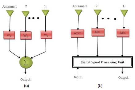
Figure 1 (a). Analog Beam forming (b) Digital Beam forming

The explosive growth in the demand for wireless communication using handsets and personal communication devices has created the need for major advancements of antenna design as a fundamental part of any wireless systems [4]-[7]. Added to the operational requirements, the user and service providers demand wireless units with antennas that are small and compact, cost effective, low profile and easy to integrate with the wireless communication system [8]-[10].

A smart antenna is aided by some smart algorithm designed to adapt to different signal environments. With the help of associated hardware and a computer controller, a smart antenna changes the array pattern in response to the radio frequency environment. Thus it can mitigate fading through diversity reception and beamforming [11].

Modern smart antenna systems still continue using the previously described techniques but taking advantage of digital signal processor [12]. The signal processing is performed at base band instead of doing it at RF stage. More new beamforming techniques have emerged based on digital signal processing [13].

The convergence of the adaptive algorithm is directly proportional to the step-size parameter μ. If the step-size is too small, the convergence is slow and we will have the over damped case. If the convergence is slower than the changing angles of arrival, it is possible that the adaptive array cannot acquire the signal of interest fast enough to track the changing signal. If the step-size is too large, algorithm will overshoot the optimum weights of interest. This is called the under damped case. One of the drawbacks of the LMS adaptive scheme is that the algorithm must go through many iterations before satisfactory convergence is achieved. If the signal characteristics are rapidly changing, the LMS adaptive algorithm may not allow tracking of the desired signal in a satisfactory manner [3], [14] .

In this work, the authors have analyzed the performances of both normal LMS and NLMS algorithms. Since both the algorithms show significant interferences and slow convergence speed, these downsides, limits LMS and NLMS applications for high speed advanced cellular communications. The proposed VSSNMLS overcomes the limitations of these methods.

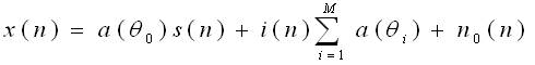
Let us consider system model with a Uniform Linear Array (ULA) consisting of 'L' isotropic sensors. Let 'm' (m < L be the unconstrained signals impinging on a ULA at directions θ₁ , θ₂ ... θ_m ). Consider 'd' as inter element spacing of ULA and its value chosen to be λ/2 in order to reduce mutual coupling effects. The narrowband signal received by a linear antenna array with L - Omni-directional antenna elements at the time instant n can be expressed as [14].

(1)

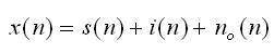
Where s(n), i(n) and n₀(n) denote the N×1 vectors of the Signal of Interest (SOI), interference and noise respectively. For simplicity, all these components of the received signal are assumed to be statistically independent to each other. This assumption is fairly practical since the SOI and the signals from interferers (other objects or users) are typically independent. The conventional (forward-only) estimate of the covariance matrix defined as, R=E{x(n)x^H (n)}=σ²I, where σ² is the noise power at a single antenna element, I denotes the identity matrix and (•) H and E [•] stand for the Hermitian transpose and mathematical expectation respectively. Figure 2 shows the L-element antenna array.

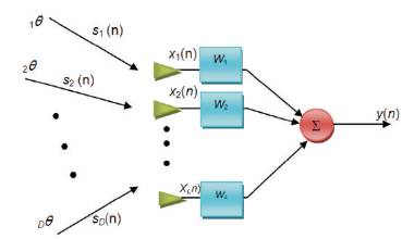
Figure 2. L-element Antenna Array with Arriving Signals

2.1 Least Mean Square (LMS) Algorithm

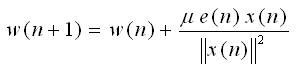
The convergence speed of an algorithm is an important property, and its significance for mobile communications is highlighted in [2] by illustrating how the normal LMS beamformer does not perform well due to its slow convergence rate in environment of fast-changing signal characteristics. The availability of required time for an algorithm to converge in cellular communications system depends not only on the design of system, which dictates the time of the user signal present (such as the user duration in a TDMA based system) but also on the speed of mobile phones, which changes the rate at which a desired signal fades. The weight update equation of steepest decent method is given by,

(2)

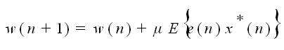
Where, E is the expectation operator, m is the step size used for convergence of beam forming algorithm, e(n) is the * error signal and x (n) is the conjugate of induced signal.

2.2 Normalized Least Mean Square (NLMS) Algorithm

The main drawback of the normal LMS is its slow convergence rate. This makes it very difficult to choose a step size μ that guarantees stability of the LMS. The NLMS algorithm and its convergence analysis using different types of data have been studied widely [8]–[13] . It avoids the requirement for estimating the eigen values of the essential correlation matrix or its trace for obtaining of the maximum permissible step size. The NLMS has better convergence rate and less signal sensitivity as compared to the normal LMS algorithm. A discussion of its application to different wireless communications can be found in [9].

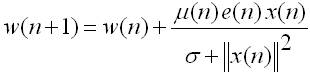
The weight for the NLMS algorithm is given by,

(3)

3.1 Variable Step Size Normalized Least Mean Square (VSSNLMS) Algorithm

The main objective of the developed VSSNLMS algorithm is to replace the fixed step size μ that is used in conventional NLMS by a variable one. This is to nullify a trade-off issue between steady-state MSE and convergence rate. A large step size is used in this algorithm in the initial stages to speed up the convergence rate and a smaller μ is used near to the steady state of the MSE to achieve an optimum value. Figure 3 shows the flow diagram of this method. Let 'D' is number of user signals coming from different directions. In a practical case, if s(n) is the signal samples corresponding to look direction , i(n) is interfering signal samples corresponding to jamming directions and n₀(n) is noisy signal samples due to receiver components. The induced signal is given by,

(4)

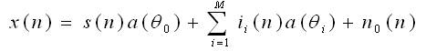
Where, M is number of jamming sources, a(θ₀) is desired steering vector and a(θ_i) is the steering vector corresponding to i^th interference signal.

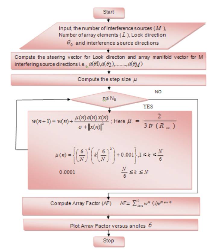
Figure 3. Flow Diagram of the Proposed VSSNLMS Algorithm

Since jamming signals (or interfering signals) are of no interest, it is assumed i(n)₁ = i(n)₂ ......i(n) _m = i(n) with this above equation can be written as,

(5)

In matrix notation, induced signal can be written as,

(6)

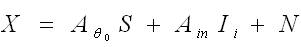
Where, X represents L x N_s induced signal matrix, N_s is total number of samples, 'L' represents number of array elements, ‘S’ represents reference signal samples. is the desired steering vector of order Lx1, I_i represents the interference signal samples matrix of order 1xN_s , N represents Gaussian noise matrix of order LxN_s and A_in is Lx1 column vector.

(7)

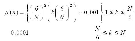
The step size varied for the various iterations is given by the equation,

(8)

Thus, the array output y can be expressed as,

(9)

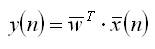
and the error signal is calculated as, e(n)=s(n)-y(n).

The proposed VSSNLMSS algorithm is simulated using MATLAB software. The parameters used in the simulations are tabulated in Table 1.

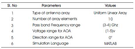
Table 1. Parameters used in the Simulation

Figure 4 shows the amplitude of the desired signal and its variation as a function of number samples. Figures 5 and 6 show the noise signal amplitude for various samples and signal step size amplitude as a function of various iterations respectively. Figure 7 shows the curve function plot, Figure 8 shows the error performance of VSSNLMS, Figure 9 shows the normalized array power pattern. Figures 10 and 11 show the ration pattern of VSSNLMS in rectangular and polar form respectively.

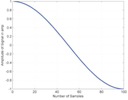
Figure 4. Amplitude of Desired Signal

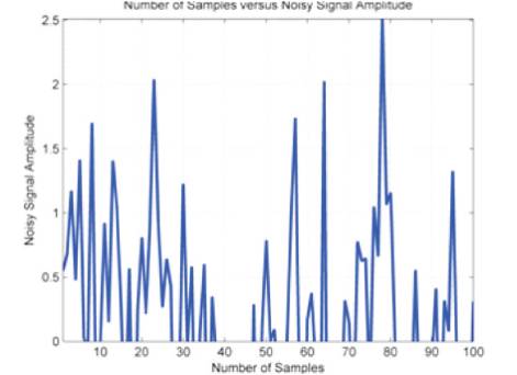
Figure 5. Amplitude of Noisy Signal

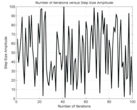
Figure 6. Amplitude of Step Size

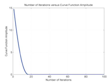
Figure 7. Curve Function of VSSNLMS Algorithm

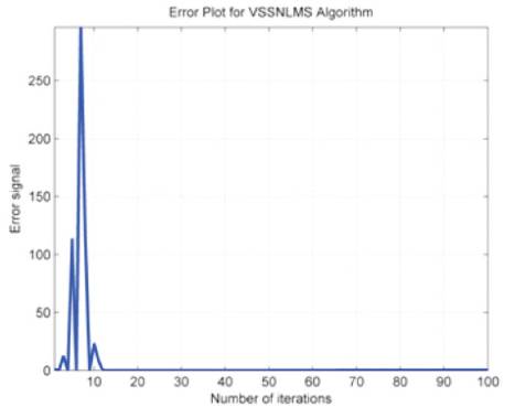
Figure 8. Error Performance of VSSNLMS

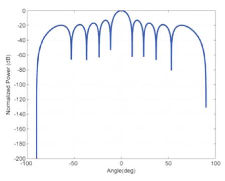
Figure 9. Normalized Power Pattern of VSSNLMS Algorithm

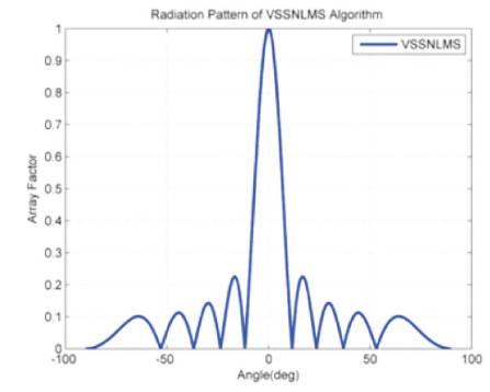
Figure 10. Rectangular Radiation Pattern of VSSNLMS

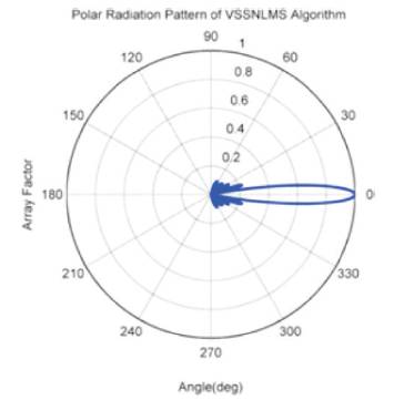
Figure 11. Polar Plot of VSSNLMS

Let us consider six interference signals are obtained from angles - 60^o ,-40^o ,-20^o , 20^o , 40^o and 60^o . The Normal LMS and NLMS uses fixed step size, whereas variable step size is used for the proposed VSSNLMS algorithm. Figure 12 shows the normalized beam pattern of LMS, NLMS and VSSNLMS algorithms respectively to study the depth of null. Table 2 shows the null depths of the three algorithms.

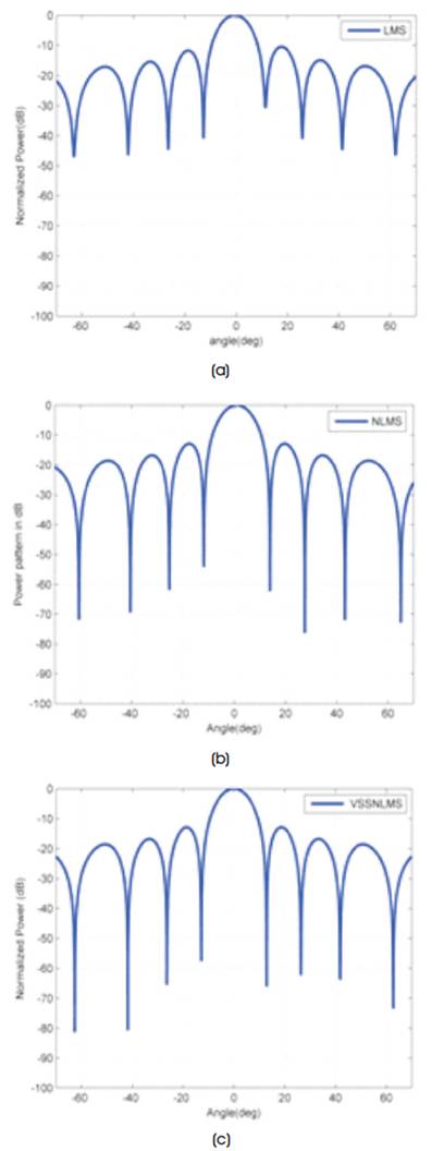
Figure 12. Comparison of Normalized Beam Pattern using (a) LMS, (b) NLMS and (c) VSSNLMS Algorithm

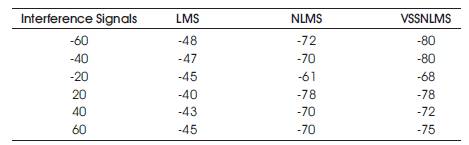
Table 2. Normalized Power in DB of Selected Nulls

The Comparison of LMS, NLMS, and VSSNLMS algorithms with respect to MSE v/s number of iterations is shown in Figure 13. From Figure 13, it is clear that the proposed VSSLMS algorithm has an improved convergence rate as compared to the normal LMS and NLMS algorithms. Hence, VSSNLMS algorithm overcomes the disadvantages of LMS algorithm.

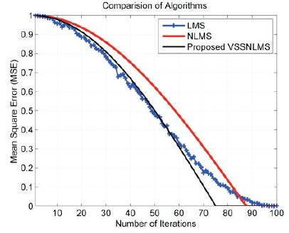
Figure 13. Comparison of Convergence Rate of LMS, NLMS and VSSNLMS Algorithms

A new robust VSSNLMS algorithm is devised for smart antenna system to improve the convergence rate and interference suppression. From Table 2 and Figure 13, it is clear that the proposed algorithm has less MSE which improves the convergence rate. It also shows the better interference suppression due to deep nulls produced in the direction of interferences. This makes the algorithm more suitable for mobile communication applications where the signal characteristics changes rapidly.