This Paper deals with the control of chaotic dynamics of healthy, infected CD+4 T-cells and free HIV (Human Immunodeficiency Virus) cells in a chaotic system of HIV infection of CD+4 T-cells by implementing a Lie algebraic exact linearization technique. A nonlinear feedback control law is designed, which induces a co-ordinate transformation thereby changing the original chaotic HIV system into a controlled linear system. Numerical simulation has been carried by using Mathematica that witness the robustness of the technique implemented on the chosen chaotic system.
The stabilization and control of chaotic systems have significant applications in nonlinear sciences. Chaos control has been an active research topic since the nineties. Due to the complexity of chaotic systems, it is hard to develop a particular suitable method to justify the design of these kind of controllers. Specially, after OGY (Ott Grebogi and Yoke) method [1] , chaos control has given rise to many applications including chaotic lasers, stabilizing cardiac rhythms, biological, artificial neural dynamics and autonomous robot control [2-4]. Among many developed techniques for control (suppression) of chaos, some of them are Melnikov's method [5], controlling chaos through perturbation in Hamiltonian dynamics using inversion formula [6,7]. There is another successful technique based on Lie algebra in which, the chaotic system is transformed into an equivalent linear system through invertible coordinate transformation without loss of generality [8- 15]. Motivated by the aforecited studies, the author aims to control the chaotic dynamics of HIV infection of CD+4 T- cells system using Lie algebraic exact linearization technique. The main advantages of this approach is that, it is not only robust but also in + this approach, the control is injected only on infected CD +4 T-cells (i.e, I(t)) and the effect of control can be seen on the rest of state variables (i.e. T(t) & V(t)).
Rest of the paper has been organized as follows: In section 1, a brief methodology has been described, whereas section 2 is on problem formulation. Section 3, contains the implementations of the technique on the considered system. Section 4, is based on numerical simulations and lastly the whole study has been concluded.
It is a technique of controlling a chaotic system that involves transformation of a given nonlinear system into a linear system by injecting a suitable control input [8]. Let us consider a non-linear dynamical system as,

After injecting the control term, it can be written as,
where,
x ∈ Rn is the state vector;
u ∈ R is the control parameter,
f : Rn → Rn and g : Rn → Rn are both smooth vector fields on Rn .
Note:
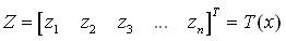
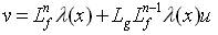
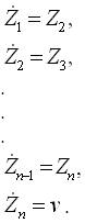
The system (equation (2)) is called as a feedback linearizable in the domain Ω∈Rn , if there exists a smooth reversible change of coordinates z = T(x), x∈Ω and a smooth transformation feedback, then
where,
v ∈ R is the new control if the closed loop system is linear [9].
For two vector fields f(x) and g(x), the different order Lie brackets are denoted by the symbols as follows:
with
and each of
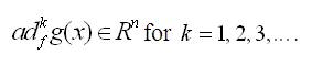
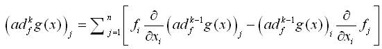
If we write,

then, (ad kf g(x))j is computed by the formula:
In some neighborhood N(x0 ) of a point x0 , if the matrix,

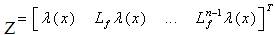
Equation (9) has a rank n and S = span { g, ad f g,ad2f g,...,adf n-2 g } is involutive, then there exists a real valued function λ(x) ∈ N(x0) , such that:
 where
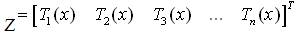
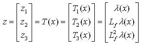
where  denotes the Lie derivative of the real valued function λ(x) with respect to the vector field F. If that happens there exists transformation in N (x0), given by:
and
that transforms the non-liner system into the linear controllable system [11, [16-18]].
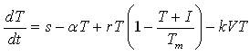
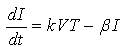
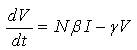
Now, the author introduces the model of HIV infection of CD +4 T-cells. The chaotic system is described by the following set of ODE (Ordinary Differential Equation) [19] as,
where,
T(t): The concentration of healthy CD+4 T-cells at time t,
I(t): The concentration of infected CD+4 T- cells,
V(t): The concentration of free HIV at time t,
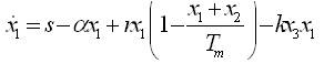
S : The source of CD+4 T-cells from precursors,α: The natural death rate of CD+4 T-cells (αTm >s),
r : The growth rate,
Tm : The carrying capacity,
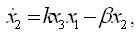
k: The rate of infection of T-cells with free virus,
β: Blanket death term for infectedcells, to reflect the assumption that we do not initially know whether the cells die naturally or by bursting,
N: Viralparticles are released by each lysing cell, this term is multiplied by the parameter N to represent the source for free virus (assuming a one-time initial infection),
γ: The loss rate of virus.
Throughout this paper, the authors set the values of the system parameters [19]: s=0.1; α=0.02; β=0.3; r=3; γ=2.4; k=0.0027; N=10; Tm =1500 with the initial conditions: T(0) =0.001; I(0)=0.01; V(0)=0.001.
Taking x1 =T; x2 =I and x3 =V, the HIV infection of T-cells can be written as:
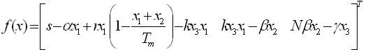
The system of equations (18-20) can be written as,

where,
and,
Parametric entrainment control u(x1 , x2 , x3 ) is applied to the parameter b in the second equations (18-20) of the system and one gets,
where,
and u ∈ R.
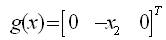
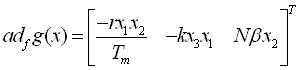
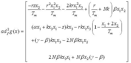
Using equations (18-20) and (24), and using a Lie bracket,
For any ,  there exists an open set N(x0) containing x0 where the matrix,
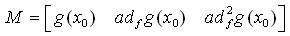
Equation (28) has rank 3 and S = span {g, ad ƒ g } is involutive.
Proof:
Let
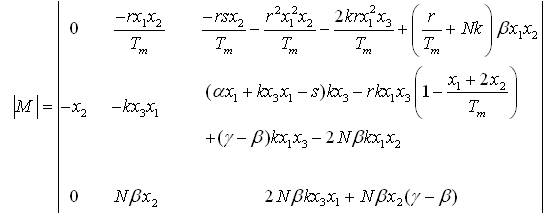
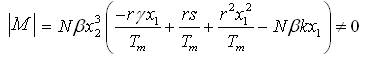
for non-zero values of state variables involved in |M|.
Therefore ρ(M)=3 or equal to the order of the system. With the help of (24) and (26) one can show that,
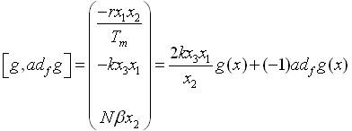
Equation (31) shows that [g, ad ƒ g] belongs to S = span {g, ad ƒ g } . Hence, S is involutive.
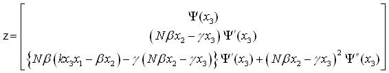
For any thrice differentiable function ψ(x3), there exists, a smooth transformation 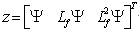 with a smooth inverse, defined in an open set N(x0) where
  that reduces system (equations 18-20) to a linear controllable form.
Proof:
Since lemma 1 holds, there exists a real valued function λ(x) such that, Lg λ(x)=0 and Lodfg λ(x)=0 but, Lod2fg λ(x)≠0. Now, Lg λ(x)=0 implies  and
and 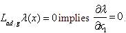 . Hence λ(x) is independent of x1 and x2 but depends on x3.
Thus,
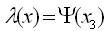
where, simple calculations yield,

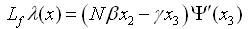
where x3 & x2≠ 0 or x1 & x2≠ 0. With the help of equation (32), one can easily calculate the following Lie derivatives given as,
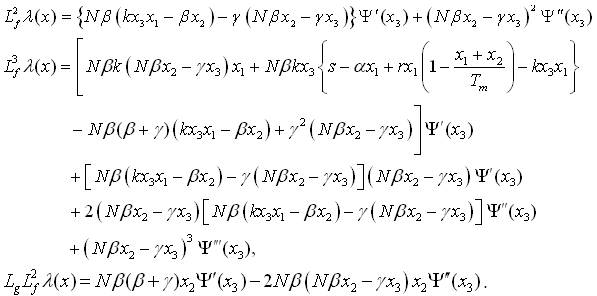
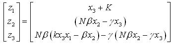
With the help of equation (35) the transformation formula (equation12) takes the form
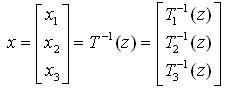
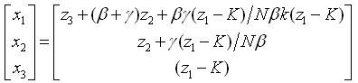
Inverse transformation can be calculated from equation (37) as,
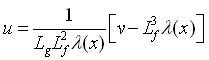
Controller u is obtained from the formula (equation 12) as
These will change the HIV infection of CD+4 T- cells system (equation 20) into a linear controllable system:

where,
v is considered linear in z1,z2 and z3.
Without loss of generality, one may choose the linear form of v as  , where,
  .
.
The controller stabilizes the equilibrium point z=(0,0,0) if a1, a2,a3 < 0 and a1+a2a3 > 0.
The controller stabilizes the system on to a stable limit cycle if a1, a2,a3 < 0 and a1 +a2a3 > 0 .
Note:
The proof of the theorems 1 and 2 can be found in [8] .
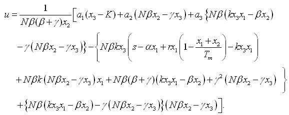
Now, using equations (35) and (39), the controller u can be written as:
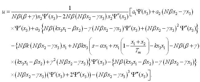
The system (equation 20) with an output function ψ(x3) becomes controlled when thecontrol loop is closed with control input given by equation (41).
Now, the problem is studied for the particular forms of ψ (x3). However, there are many choices for ψ(x3) (i.e. linear, quadratic, etc. in x3 ). Here, the author chooses only linear because the other kind of forms will give more complicated forms of u after tedious calculations.
Let, a linear output ψ(x3)=x3-xg will give control law:
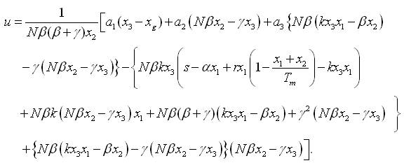
Equation 42, stabilizes system (equation 20) to the control goal
where,
xg is the parameter that determines the control goal.
Let,
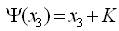
where,
K is arbitrary constant to be determined later.
Controlling the system (equation (41)) to the origin and changing the values of K, one can control x to the control goal xg . In this case control law takes the form
For the transformations, from linear to nonlinear and vice-versa, we have the following relations respectively,
Since, the feedback control law stabilizes the equilibrium point of (equation (40)), then using equation (21) and changing the value of K, one can control x3 to the goal xg and the variation of K is given by the formula

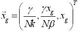
As x3 goes to the goal xg , the state vector x goes to 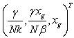
The system parameters involved in equation (20) has been taken as: s=0.1; α=0.02; β=0.3; r=3;
γ =2.4; k=0.0027; N=10; Tm =1500 with the initial conditions: T(0)=0.001; I(0)=0.01; V(0)=0.001, and for K=10; a1 =-0.1; a2 =-0.2, a2 =-0.6 a controller is given by equation (45), is evaluated. Using Mathematica, various graphs have been plotted to show the robustness of the implemented technique. Figures 1 and 2 depict the uncontrolled and controlled time series of the state variables of the system (equation 20) respectively, whereas the phase plots (a graph between state vector & its derivative) of three state vectors are shown in Figures 3-5 for controlled and uncontrolled one respectively. Someone observe that chaotic attractors are being replaced by regular ones as the controller is injected. Comparative parametric plots of the controlled and uncontrolled state vectors pairwise and 3D has been sketched (Figures 6- 10). The non-zero values of state variables involved in M is also confirmed by Figure 11.
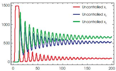
Figure 1. Time Series of Uncontrolled x1 , x2 , and x3
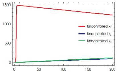
Figure 2. Time Series of Controlled x1 , x2 , and x3
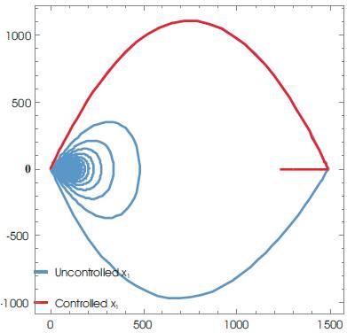
Figure 3. Phase Plots of x1
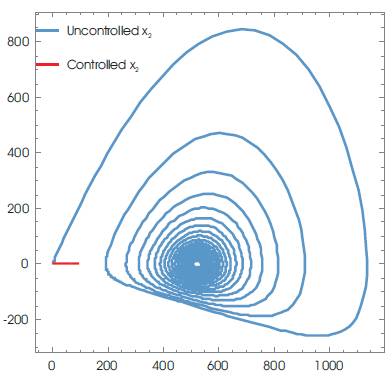
Figure 4. Phase Plots of x2
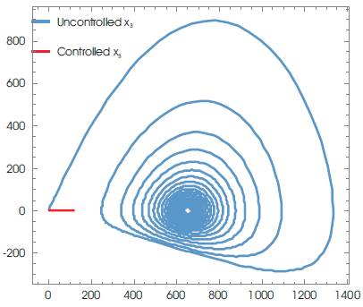
Figure 5. Phase Plots of x3
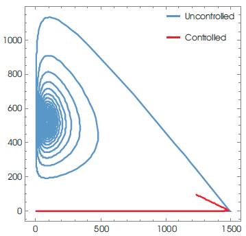
Figure 6. Parametric Plots between x1 and x2
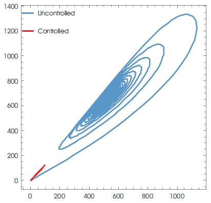
Figure 7. Parametric Plots between x2 and x3
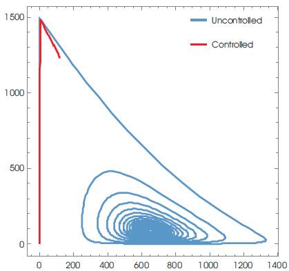
Figure 8. Parametric Plots between x3 and x1
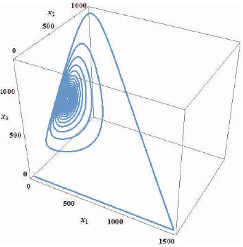
Figure 9. Parametric 3D plot of uncontrolled State Vectors
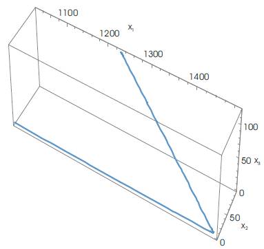
Figure 10. Parametric 3D plot of controlled State Vectors
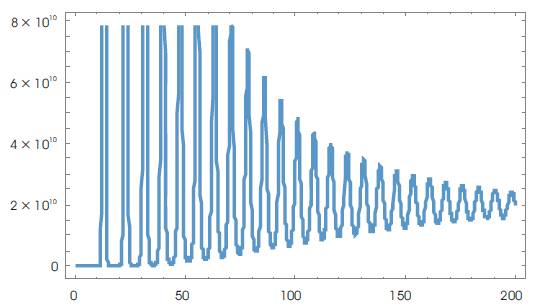
Figure 11. Time Series of Det (M)
In this paper, the author has controlled the chaotic dynamics of HIV infection CD+4 T-cells system using the exact linearization method based on Lie algebra. Without the loss of generality, an equivalent linear system to the considered chaotic system has been obtained using Lie algebra. Also, a single control term has been injected to the chaotic system and the control has been observed in all three state vectors representing the concentration of healthy CD +4 T-cells (T), infected CD+4 T- cells (I), and free HIV (V) at time t. The control and robustness of the technique can be seen in Figures 1-10.