Electromagnetic transients in Electric Power Systems (EPS) are common, and are in general induced by short circuits, switching operations and lightning cases. These events can be permanent or non permanent to the EPS. In both cases, however, the occurrence of such events constantly implies the protection relays operation to isolate the correct faulted equipment. After the protection scheme operation, the faulted equipment can be restored. Permanent faults, however, need to be detected and located first, in order to send maintenance crews to fix the equipment [16, 17]. Restoration of faulted equipments can generate the reoccurrence of the fault, resulting into power system blackouts. In the modern electrical power systems of transmission and distribution systems, underground cable is used largely in urban areas and compared to overhead lines, fewer faults occur in underground cables. However in high power distribution system with underground power cables, in case faults take place, it becomes highly intricate to performing fault localization and repair. Underground cables have been widely applied in power distribution networks due to the benefits of underground connection, involving more secure than overhead lines in bad weather, less liable to damage by storms or lightning, no susceptible to trees, less expensive for shorter distance, environment-friendly and low maintenance. However, the disadvantages of underground cables should also be mentioned, including 8 to 15 times more expensive than equivalent overhead lines, less power transfer capability, more liable to permanent damage following a flash-over, and difficult to locate fault. On the basis of broad category, faults in underground cables can be normally classified as, incipient faults and permanent faults. Usually, incipient faults in power cables are gradually resulted from the aging process, where the localized deterioration in insulations exists. Electrical overstress in conjunction with mechanical deficiency, unfavorable environmental condition and chemical pollution, can cause the irreparable and irreversible damages in insulations. In general, there are three predominant types of faults in underground power cable; these are single phase-toearth (LG) fault; double phase-to-earth (LLG) fault and three phase-to-earths (LLLG) fault. The single line to earth fault is the most common fault type and occurs most frequently. Fault detection and location based on the fault induced current or voltage travelling wave[12] has been studied for years together. In all these techniques, the location of the fault is determined using the high frequency transients. Fault location based on the travelling waves can generally be categorized into two: single-ended and double ended. For single-ended, the current or voltage signals are measured at one end of the line and fault location relies on the analysis of these signals to detect the reflections that occur between the measuring point and the fault [4, 5, 9, 13]. For the doubleended method, the time of arrival of the first fault generated signals are measured at both ends of the lines using synchronized timers.

In general, many authors have done research work for fault detection and location by some methods like impedance method, online method single end and double end method, transient wave method, etc., but the accurate measurement is very essential for proper erection or repair of underground cable and to have restored of electrical energy as quickly as possible. As per the literature survey, it is observed that wavelet transform is a powerful tool box for high frequency non stationary signals. Performing the comparison of the transient signals at all phases in power cable model, the classification of fault can be made. If the transient signal appears at only one phase, then the fault is single line to ground fault (if appears at two phases - LLG, appears at three phases - LLLG fault). In general, the generated transient signals caused due to the fault is found to be non-stationary and is of wide band of frequency, when fault occurs in the network, the generated transient signals travels in the network [10,11]. On the arrival at a discontinuity position, the transient wave is in general, reflected partly and the remainder is incident to the line impedance. The transient signals reflected from the end of the line travels back to the fault point where another reflection takes place due to the discontinuity of impedance.

In the proposed fault identification and localization scheme, wavelet scheme has been employed in order to capture these transient signals since the wavelet transform can extract the non stationary high frequency signals and can give accurate transient information. The wavelet coefficients have been used for fault location in the proposed system. The fault location can be carried out by comparing the aerial mode wavelet coefficient to determine the time instant when the energy of the signal reaches its peak value. The distance between the fault point and the bus of the faulted branch is in general stated by the following equation (1).

(1)

where D represents the distance to the fault, t_d refers for the  time difference between two consecutive peaks of the wavelet transform coefficients of the recorded current and v is the wave propagation velocity in the aerial mode. An underground cable of length 200 km has been employed for fault analysis. The travelling wave velocity of the signals in the 11kV underground cable system is  1.9557x10⁵ km/s, and sampling time of 10μs has been employed. Figure 1 represents the single line diagram of 11kV, 50Hz, 200km three phase underground power cable, where X₁ is the distance to fault point from the  source and t. Figure 2 shows the Proposed System.

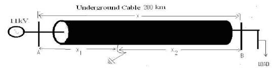
Figure 1. Single Line Diagram of Three Phase -11kV, 200km Underground Cable

Figure 2. Configuration of Proposed System

To perform the system analysis, varied fault conditions such as LG, LLG and LLLG faults have been considered and associated detection parameters have been obtained. The performance has been evaluated in terms of % error and the deviation from the actual values. The overall process of fault detection and location has been accomplished. Consider a three phase cable line of length X connected between bus A and bus B, with characteristic impedance Z_c and traveling wave velocity  of v. In this simulation model, it has been found that, if a fault occurs at a distance X₂ from bus A, this will appear as  an abrupt injection at the fault point. This injection will travel like a wave "surge" along the line in both directions and will continue to bounce back and forth between fault point, and the two terminal buses until the post- fault steady state is reached. The distance to the fault point can be calculated by using travelling wave theory. Let t₁ and t₂ corresponds to the time at which the modal signals  wavelet coefficients in scale 1 show their initial peaks for signals recorder at bus A and bus B respectively. The delay between the fault detection times at the two ends is (t₁ - t₂)   can be determined. Once the parameter t_d is  determined, the fault location from bus A can be estimated as per the following expression (2).

(2)

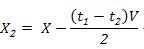
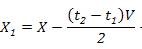
Or the fault location can be calculated from bus B as follows expression (3)

(3)

The travelling wave velocity can be obtained from the equation as follows (4)

(4)

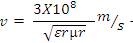
Here v is assumed to be 1.9557x10⁵ km/s, with sampling time of 10μs and the total line length 200km. In the above mathematical model, the variable X₁ and X₂ represents the distance to the fault, t_d is the time difference between  two consecutive peaks of the wavelet transform coefficients of the recorded current and v is the wave propagation velocity.

A wavelet is a mathematical function[1, 2, 6] used to divide a given function or continuous-time signal into different scale components. Usually one can assign a frequency range to each scale component. Each scale component can then be studied with a resolution that matches its scale. A wavelet transform is the representation of a function by wavelets. The wavelets are scaled and translated copies (known as "daughter wavelets") of a finite-length or fast-decaying oscillating waveform (known as the "mother wavelet"). Wavelet transforms have advantages over traditional Fourier transforms for representing functions that have discontinuities and sharp peaks, and for accurately deconstructing and reconstructing finite, non-periodic and/or non-stationary signals. Wavelet transforms are classified into Discrete Wavelet Transforms (DWTs) and Continuous Wavelet Transforms (CWTs). In the wavelet transform it is noted that, both DWT and CWT are continuous-time (analog) transforms. They can be used to represent continuous-time (analog) signals [14]. CWTs operate over every possible scale and translation whereas, DWTs use a specific subset of scale and translation values or representation grid.

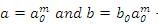
The wavelet transform can be accomplished in two different ways depending on what information is required out of this transformation process [6, 7]. The first method is a Continuous Wavelet Transform (CWT), where one obtains a surface of wavelet Coefficients, [1, 2] CWT (b,a), for different values of scaling 'a' and translation 'b', and the second is a Discrete Wavelet Transform (DWT), where the scale and translation are discredited, but not are independent variables of the original signal. In the CWT the variables 'a' and 'b' are continuous. DWT [6, 7] results in a finite number of wavelet coefficients depending upon the integer number of discretization step in scale and translation [14, 15] denoted by 'm' and 'n'. If a₀ and b₀ are the segmentation step sizes for the scale and translation respectively, the scale and translation in terms of these parameters will be,

(5)

(6)

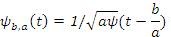
The above presented equation represents the mother wavelet of continuous time wavelet series. After discretization in terms of the parameters, a₀ , b₀ 'm' and 'n',  the mother wavelet can be written as,

(7)

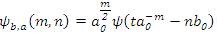
After discretization, the wavelet domain coefficients are no longer represented by a simple 'a' and 'b'. Instead they are represented in terms of 'm' and 'n'. The discrete wavelet coefficients DWT (m, n) are given by the equation:

(8)

The transformation is over continuous time, but the wavelets are the transformation is over continuous time but the wavelets are represented in a discrete fashion. Like the CWT, these discrete wavelet coefficients represent the correlation between the original signal and wavelet for different combinations of 'm' and 'n'.

Wavelets equal to the second derivative of a Gaussian function are called Mexican Hats (MH). They were first used in computer vision to detect multi scale edges. Figure 3 shows the MH Wavelet Transforms. The MH Wavelet family is given by the following equations

(9)

(10)

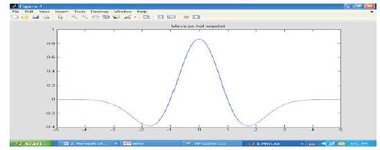
Figure 3. Mexican Hat Wavelet Transforms

This is obtained by taking the second derivative of the Gaussian function. The Mexican hat wavelet is not the only kind of analysing wavelet.

In the proposed system, all the possible cases of ground faults are selected to illustrate the performance of the proposed technique under fault conditions the fault location for LG at 25km and 50km, Figure 4 and Figure 5 show the current response for LG fault at 25km as well as 50km respectively. From the figures, it can be observed that, due to the fault the current signals gets distorted and there is rise of fault current and moreover the fault current magnitude is more for fault at 50km than the fault at 25km from the source.

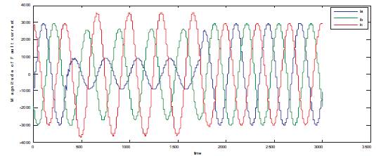
Figure 4.Current Response for LG Fault at 25 km

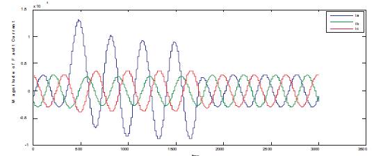
Figure 5. Current Response for LG Fault at 50km

In the next stage of the research work, the simulation work has been carried for double line to ground fault (LLG) both at 25km and 50km respectively. Figure 6 and Figure 7 show the current response for double line to ground fault (LLG) at 25km and 50km respectively. From Figure 6 and Figure 7, it can be observed that, two phases of three phases gets distorted and the fault current magnitudes have been changed compared to the previous case of study.

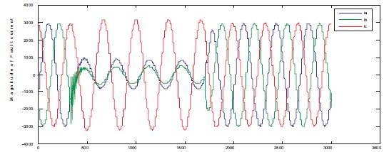
Figure 6. Current Response for LLG Fault at 25km

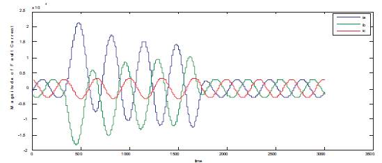
Figure 7. Current Response for LLG Fault at 50km

In further stage of the proposed work, the simulation work has been carried for three phase to ground (LLLG) fault both at 25km and 50km respectively. Figure 8 and Figue 9 show the current response for three phases to ground (LLLG) fault for 25km and 50km respectively. From Figure 8 and Figure 9, it is observed that, all the three phase current were distorted and the magnitude of fault current has been furtherly changed when compared with above two cases of current study.

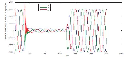
Figure 8. Current Response for LLLG Fault at 25km

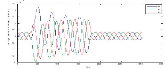
Figure 9. Current Response for LLLG Fault at 50km

From the outcomes, the fault location has been estimated using the following formulae as shown in equation (12).

(11)

In the process of identification of fault location, the simulation work has been carried by the impedance method and the outcome is compared with the actual location of fault. Table 1 shows the percentage of error in km, from the Table 1, it can be observed that, the fault point estimated by impedance method for fault at 25km for LG fault is 29km, for LLG 23.12km and for LLLG is 31.22km, i.e there is error of -4%in case of LG fault, 1.88% in LLG fault case and -6.22% in LLLG fault condition when compared with the actual distance of fault and is shown in Table 1 and Table 2.

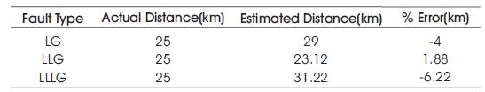
Table 1. % Error by Conventional Method for 25km

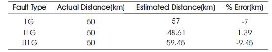
Table 2. % Error by Conventional Method for 50km

In the next stage of the research work, wavelet transforms technique[1, 2] chosen as the wavelet transform is a very powerful tool for high frequency non stationary signals as well as the fault signals. There are many wavelet families; however the selection of suitable wavelet plays an important role in the accuracy of the outcomes. In the proposes work discrete wavelet transform methods [6, 7] has been selected as the fault concern to high frequency and there may be discontinuity in the signal which is to explored for extraction of high frequency signals. According to the efficiency of extraction of high frequency signals and type of wavelet selection. In the proposed work, Mexican Hat and Coif Let wavelet transforms are chosen for the detection and location of faults, since Mexican Hat and Coif Let transform gives the better result. Figure 10 shows the overall flowchart of the proposed work. The flowchart gives the information about the procedure how the fault detection and localization can be done very clearly.

Figure 10. The Overall Flowchart of the Proposed Algorithm

LG fault is selected as simulation case and fault locations are tabulated along with % error to compare the deviation from the actual values using wavelet transform (Mexican hat and coif let) and similarly in the second stage LLG fault is selected and in the final stage LLLG fault is selected. The simulated results of the proposed system are shown in Figures 11 to 22, for both 25km and 50km fault points. The results are obtained from the impedance method and the wavelet transform (Mexican hat and coif let) are compared with actual distance and are tabulated in Tables 3, 4, 5 and 6. From the outcomes of the proposed system, it is found that the proposed algorithm can detect fault with an accuracy of 100%. As a result, it is found that, the application of the wavelet transform (Mexican hat and Coif Let) is a good choice in detecting and locating the fault points in underground cables accurately.

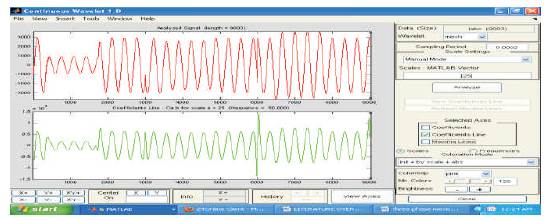
Figure 11. Current Response for LG Fault at 25 km (Mexican Hat)

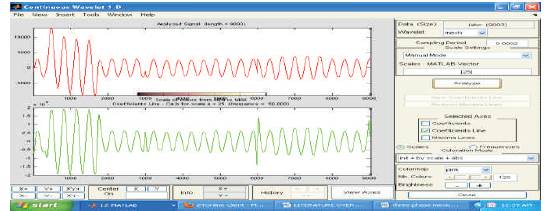
Figure 12. Current Response for LG Fault at 50km (Mexican hat)

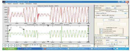
Figure 13. Current Response for LLG Fault at 25 km (Mexican Hat)

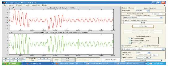
Figure 14. Current Response for LLG Fault at 50 km (Mexican Hat)

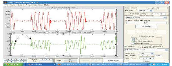
Figure 15. Current Response current for LLLG Fault at 25 km (Mexican Hat)

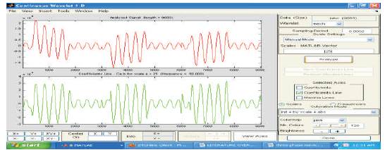
Figure 16. Current Response Current for LLLG Fault at 50 km (Mexican Hat)

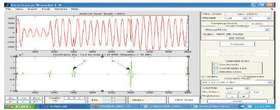
Figure 17. Current Response for LG Fault at 25 km (Coif Let)

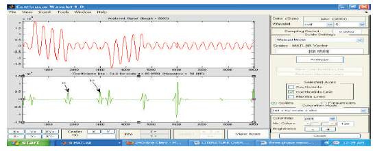
Figure 18. Current Response for LLG Fault at 25 km (Coif Let)

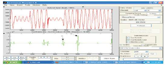
Figure 19. Current Response for LLG Fault at 25 km (Coif Let)

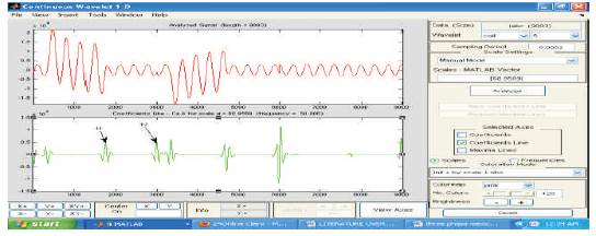
Figure 20. Current Response for LLG Fault at 50 km (Coif Let)

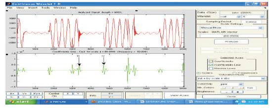
Figure 21. Current Response for LLLG Fault at 25 km (Coif Let)

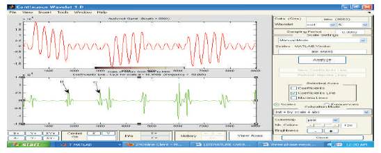
Figure 22. Current Response for LLLG Fault at 50 km (Coif Let)

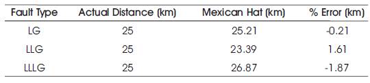
Table 3. % Error by Mexican Hat Wavelet Transform for 25km

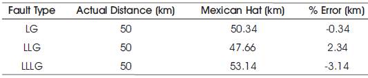
Table 4. % Error by Mexican Hat Wavelet Transform for 50km

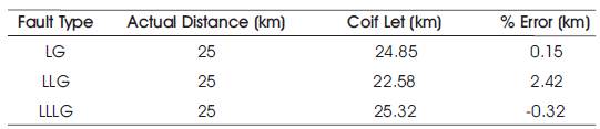
Table 5. % Error by Coif Let Wavelet Transform for 25km

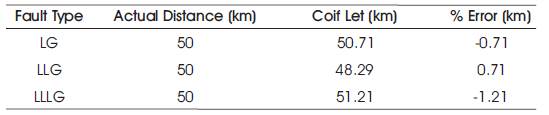
Table 6. % Error by Coif Let Wavelet Transform for 50km

In the next stage of the proposed work, the fault current responses caused by single line to ground fault (LG), double line to ground fault LLG) and triple line to ground fault (LLLG) are explored to the Mexican Hat and Coif let wavelet transform for extraction of signals. The Mexican Hat wavelet transform has been performed at scale of 25; sampling period of 20ms and the high frequency non stationary fault transient signals have been converted into 50Hz signal. Figure 11and Figure 12 show the outcome of the Mexican hat and Coif Let wavelet transforms for LG faults at 25km and 50km respectively. From Figure11 to Figure16, it can be observed that the peaks which indicate the arrival of fault, considering the first two peaks the distance of fault can be evaluated. The number of peaks in figures indicates the type of fault.

From the outcomes of the Mexican hat wavelet transforms, the location of fault have been evaluated for LG, LLG and LLLG faults for both at 25km and 50km respectively are shown in Table 3 and Table 4.

From the Table 3 and Table 4, it can be observed that, the actual LG fault location is 25km, the evaluated location by Mexican Hat is 25.21km and for 50km fault, it is 50.34km i.e. there is an error of -0.21 % and -0.34% for 25km and 50km respectively. Similarly for LLG fault evaluated location is 23.39km for 25km and 47.66km for 50km and an error of 1.61 % and 2.34% respectively. The same procedure has been adopted for LLLG fault also, the evaluated location for 25km is 26.87km for 25km and 53.14km for 50km and resulted a error of -1.87% and - 3.14%. In the next stage of the proposed work, the fault signals have been explored to coif Let transform for extraction of transient information. The Coif Let wavelet transform has been performed at a sampling period of 20ms and a scale of 68.9569 and the high frequency non stationary transient signals converted in to 50Hz signals. The outcomes of coif let wavelet transform for LG, LLG and LLLG faults are shown in Figure 17 to Figure 22. From the Figure 17 to Figure 22, it can be observed that there is peak changes in the response and which indicates the type of fault, the location of fault can be evaluated by the arrival of peaks.

The Coif Let wavelet transform outcomes are noted and they are tabulated in Table 5 and Table 6.

From the Table 5 and Table 6, it can be observed that, the actual fault location is 25km, the evaluated location by Coif Let transform is 24.85km and for 50km fault, it is 50.71km i.e. there is an error of 0.15% and -0.71% for 25km and 50km respectively. Similarly the evaluated location for LLG fault at 25km and 50km are 22.5km and 48.29km and it exhibits an error of 2.42% and 1.71% respectively. The same procedure as been adopted for LLLG fault and the evaluated results are 25.32km and 51.21km for 25km and 50km and exhibits an error of -0.32% and -1.21% respectively.

The aim of this research presents a reliable method for detection and localization of faults in underground power cable. The proposed method of detection and localization is very powerful tool, as it extracts the high frequency signals and gives the transient information inters frequency and time domain, which misses no time components and frequency components as in the case of FFT and time domain analysis. In the proposed research work,11kV.500MVA, 200km length cable has been tested with all possible ground faults and location of fault has been estimated with impedance method as well as wavelet transform (Mexican Hat and Coif Let) used for location of faults. The Mexican Hat transform performed at sampling period of 20ms and at a scale of 25, Coif Let transform is performed at sampling period of 20ms and at a scale of 65.9569 and by the localization of faults was performed at 25km and 50km for all possible ground faults. The outcomes of impedance method and wavelet based are compared and the percentage of error tabulated in Tables 1 to 6. The percentage of error by impedance method is very high and is very less by wavelet transform (Mexican Hat as well a Coif Let), which means it is again proved that the wavelet transform gives an accurate and exact location and can be used for location of faults in practice.

The first author would like to express her gratitude to Prof. Dr. M. Surya Kalavathi, who encouraged her to pursue this work and taught her the art of localization of faults in underground power cables using wavelet transform. It is her pleasure to acknowledge the role of her co author K. Prakasam in completion of this work.