---

The Model Predictive Control (MPC) technique determines the control effort in a receding horizon manner by minimizing the cost function by using an explicit model while satisfying the imposed constraints. The scheme was introduced by Richalet et al. [1], where the author has coined predictive control based on an impulse-response model by the name of a Model Predictive Heuristic Control (MPHC), which later became popular as Model Algorithmic Control (MAC). The model predictive controller repeatedly solves a linear programming problem while maintaining the optimal plant operation under the specified constraints on Controlled Variables (CVs), Manipulated Variables (MVs) and measured Disturbance Variables (DVs). The timedomain constraints on signals can also be handled with the ease in MPC, the basic algorithm is easy to understand and implement. It uses quadratic programming methods for solving the quadratic cost function [2-4].

However, MPC is being used to control slow dynamics i.e., for calculation of set-point for low-level controllers which indirectly control the fast dynamics of the system. Rather, it has not directly replaced the classical methods, such as PID controller. The basic linear MPC formulation does not take into account, the inherent model uncertainties whether they are due to un-modelled dynamics, disturbances or nonlinearities. The advancements in the optimization algorithms, and with the betterment of fast computation techniques now, it is easier to implement the idea of MPC in the real-time applications.

MPC provides an unambiguous model of a system, the sequence of MVs which could be vigorously updated as soon as the new observations of the CVs are available. The optimization problem is solved at each sampling instant, to maintain the CVs, MVs and the plant or process trajectory under the limits of specified constraints. The first control action of the prediction horizon is applied to the plant/process. In the next sampling period, the time horizon shift to one sample forward and the same act is repeated by the controller.

The inputs to the process are calculated to optimize the future plant performance over a specified time horizon, which is called as the prediction horizon. Today, MPC is used in a multi-level hierarchy of control functions [1]. It becomes challenging to implement the suitable control actions in a multi-level process, where various constraints are to be kept under the limits. The control over the plant is achieved as a result of a constrained optimization problem over a time span, where the variables to be minimized are function of the inputs and the outputs of the system.

The basic control law that MPC uses is optimization, and quadratic cost is always a performance measure for it. Defining positive definite matrices Q=Q^T >0 and R=T^T >0 (the performance weights), we want to minimize the cost and performance measure in infinite horizon to find the optimal control input.

The Linear Quadratic (LQ) controller provide solution to this problem in unconstrained case, while no solution exist when the problem is a constrained case problem. Let, the prediction horizon is N, now approximating the problem, with a finite horizon cost,

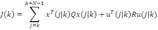
With finite horizon, the problem can be solved but it will introduce a problem in the solution itself. Let the model be,

With the current state x(k|k), the future state can be predicted, i.e., x(k+j|k), by using a future control sequence u (·|k). No state estimation is required so, x(k|k) = x (k), because we assume C=I, which gives the prediction,

The following optimization problem is defined using these predictions,

Subject to,

With this, the control algorithm steps are defined as follows:

1) Measure x(k|k)

2) Obtain u (·|k) by solving the above equation.

3) Apply u(k) = u (k|k)

4) Time update, k:=k+1

5) Repeat from step 1.

In the above optimization problem, the authors have minimized a quadratic objective which is subjected to the linear constraints. There are various efficient solution method to solve an optimization problem, and this may be a reason which made MPC so popular. The various methods are,

1. Active set method.

2. Pivoting algorithms.

3. Interior-point methods.

4. Reduced gradient algorithm.

There are various factors that affect the MPC calculation, its dynamic behaviour and calculation strategy. The models used to represent the plant or process is also a very important factor in the MPC calculation. The correct model should be tuned with appropriate tuning parameters to obtain the MVs within the constraints.

2.1 Models of the Plant

The heart of Model Predictive Control (MPC) is the process model itself. MPC requires the solutions of the model to predict the future process outputs, the form of the model selected has a large impact on the ability to implement MPC. Some specific categories of models used in MPC calculation are discussed.

2.1.1 Linear or Non-linear Models

The systems that produce the output in accordance to the principle of superposition are called linear dynamic systems. In all the control application, the linear design techniques are usually the first to be attempted and are completely satisfactory for many applications.

On the other hand, non-linear models have no specific characteristics. They can have any characteristic or demonstrate any strange behaviour. A model is nonlinear if the equations (whose solution yields the parameter estimates) of the model depend on the parameters in a nonlinear fashion. Such estimation models typically have no closed form solution and must be solved as an iterative, numerical technique.

2.1.2 Continuous – Time or Discrete – Time Models

The continuous time MPC methods successfully predict the future plant. Most of the physical laws used to develop the models are differential equations with time as an independent variable. The advantages of these methods are allowed to tune the scaling factors, poles and other parameters so that, the responses of the system can reach to the future plant as quickly as possible. For the processes that have short time constant and small sampling interval, the prediction of the continuous time MPC is not assured.

If the time space is continuous, the model is called as a continuous time model. However, if the input and state vectors are defined only for discrete instants of time k, where k ranges over the integers, the time space is discrete and the model is referred to as a discrete time model. The discrete time system evolved with the advent of digital computers, the difference equation study assumed a new significance. The representation of discrete time non-linear difference equation is done as,

2.1.3 Distributed Parameter or Lumped Parameter Models

The MPC concept is completely applicable to the systems described by distributed parameter models. In distributed parameter model, the controller uses MPC methodology to their local subsystems. The multi-level process model take information from various controllers which are implemented in it, and then use the information into their local MPC problem to co-ordinate between multi stages of the process simultaneously, and they also exchange their predictions by communication between various level of the process. Partial Differential Equations (PDE) are involved, rather than ordinary differential equations in the distributed models. The lumped models are analysed at component level and their component properties are self-contained and complete with ordinary differential equation/ differential equation based on linking component parameters for equilibrium equation.

2.1.4 Deterministic or Stochastic Models

If the results of a model are accurately determined through the equations of events and states, without any random variation, it is referred to as the deterministic model. The system model will always produce same output for a given set of input. While in stochastic models, the variables are taken over a range of values in the form of probability distributions. If the model allow us to predict the statistics of process variables based on assumptions about random effects on the models, it is a stochastic model. The explicit stochastic models provide better control in the prediction phase of MPC.

2.1.5 Input-Output or State-space Model

Input-output models provide a relation between the process input and the output, without reference to variables internal to the process. Whereas, states may be generated as mathematically convenient, intermediate variables of an input-output process model. State-space models might include equations relating to all the internal variables of the process.

The MPC algorithm uses the state- space approach, which contributes many important issues to the MPC model. The formulation leads to the natural embedding of an integral action and a simplified form for implementation of the MPC.

2.2 Selection of Tuning Parameters

The robustness of Model Predictive Controller (MPC) and its nominal stability are deeply affected by the choice of various parameters such as feedback methods, weight matrices and control horizon. These parameter which guarantee the robustness and stability of MPC are well known, for a linear system. While in the case of non-linear systems, it becomes hard to implement these parameter (zero final-state constraint, infinite horizon, etc.). Control horizon, penalty weight, prediction horizon and sampling interval are some of the most significant tuning parameters, which must be tuned appropriately to get the desired result.

2.2.1 Sampling Interval

For a stable minimum phase system, stability does not depend on the sampling interval; however, the sampling interval is kept in the range, where it can permit the on-line computations as well as adequately process the dynamics of the system/plant. Large sampling interval can result in ringing (excessive oscillations) between the sample points [5]. The robustness of an unstable system critically depends on the sampling interval chosen. In unstable systems, there exists an inverse relationship between the maximum allowable size of the sampling interval and model error. Since, feedback is only incorporated at the sampling points, the sampling interval must be chosen sufficiently small. This is a difficult design issue that has not been fully explored for nonlinear systems.

2.2.2 Prediction Horizon

Selection criteria of the prediction horizon for linear systems have been provided by various researchers [6]. But the concept becomes of much interest when it comes to nonlinear systems. Longer horizons are more sensitive to disturbances, although this effect can be partially mitigated by including a filter in the feedback loop. Nominal stability is also strongly affected by the horizon length, the horizon length shorter than the critical value produce an unstable closed loop in the system [7] .

2.2.3 Control Horizon

Linear system results indicate that shortening the control horizon relative to the prediction horizon tends to produce less aggressive controllers, slower system response and less sensitivity to disturbances [8]. The effect is very similar to that of increasing the penalty on control action in the MPC objective function.

2.2.4 Penalty Weights

For choice of weighting matrices, [9] suggested applying weights that are inversely related to the maximum acceptable range of the variables being penalized. Generally, this technique rarely provides good results because it over-penalizes control action. To provide good performance by the optimization algorithm, so applying a penalty to set point deviations that places the objective in the interval 1-100 for the range of expected conditions, and then applying small penalties (less than 10 percent of the output penalty) on control or control increments, to achieve good closed loop performance [10] gives a very good discussion on scaling issues of optimization.

2.2.5 Collocation Approximation

There are relationships between the size of the sampling interval, model error, the degree of the interpolating polynomial, and the performance and stability of model predictive control using orthogonal collocation. These relationships have not been quantified, so only heuristic guidance can be accepted. Generally, the number of collocation points should be selected 2, and should not be more than 5. Unless the model predicts rapidly varying solutions within one finite element, a smaller number is desirable to reduce the computation time.

2.2.6 Filter in Feedback Loop

Filtering the feedback signal, when using steady-state target optimization, provides good disturbance rejection and fast system response. The choice and effect of the disturbance filter is strongly system dependent. A rough measure of the effectiveness of the filter is the ratio of standard deviation with the filter to the standard deviation without the filter. The filter in the feedback loop can be effective in reducing the controller sensitivity to output disturbance; however, like other methods that slows the system response, the filter can induce unstable closed loop behaviour with unstable processes in the presence of uncertainty. Simulation studies are essential to detect such behaviour before implementations.

An amalgamated study of next generation model predictive controller is very well presented by [11] in his paper. The upcoming technologies cover the area of business and research in a well-connected fashion.

3.1 Hybrid MPC

In [12], the well-known comment was made; “processes that contain discrete components which may be different according to the process conditions, and the continuous components that are expressed by difference or differential equations of the process. Contemplation of hybrid systems that have both types of components that stimulate a rich area of research relevant to a range of important problems of control and controlling schemes in the process industries. Many plant/system theoretic concepts, as well as regulating strategies like MPC, require mending in this context”.

To have a system with more robust stability in Model Predictive Control (MPC), input-to-state stability is widely used, but it requires careful implementation when the system is discontinuous [13-14]. Various hybrid systems studies, such as illustrated by [15], partition of the state into two components, the mixed logic dynamic description, a continuous component lying in and discrete component lying in have brought up a new interesting research area. A powerful alternative is presented by [16] in which a hybrid system is described by,

An advance practical and unifying introduction to this complex area that handle with, existence of solutions, asymptotic stability, uniqueness conditions, inter alia, invariance, converse theorems and simulation is given by [16]. It ignites to influence future research on hybrid MPC.

A well defined introduction is given in [17, 4], in which an interesting area of MPC is highlighted where the control strategy is employed to reduce the complex problem of automatically synthesizing a control protocol which is expressed in temporal logic, into a set of remarkably smaller problems.

3.2 Economic MPC

Rapid response with limited overshoot to a step input and other traditional design objectives can be achieved with the adjustment of various parameters such as running cost or stage cost. But on the other hand, profitability is often the primary objective in the process industries.

In its recent development stage, Economic MPC has encountered various limitations. Some of them are stated, firstly, it is not necessary that the most profitable operation of the plant occur at an equilibrium set point; the region of most profitable operation may be anywhere in the complete cycle of the process. Secondly, the transient cost (the cost from initial state to the target state of the process) may not be optimal as the stage cost and terminal cost are not chosen to reflect the economic cost of the process. Thirdly, the dynamic model which is employed by the model predictive controller that determines an optimal equilibrium is less accurate than the steady state model of the same process. An equilibrium point determined by the latter may not be feasible for the former. The topic of economic MPC has attracted considerable attention; the work by [18] presents this area of MPC in a very well defined fashion.

3.3 Explicit MPC

The model predictive controller uses the online solution procedure to determine the control law or sequence of control laws rather than the traditional offline determination process for an optimal control problem. This is very effective in situations where an explicit solution cannot be easily calculated for the given optimal problem. With the advancement in the complexity of a process, and increased number of process steps, it is rare that an optimal control problem comes up with an explicit offline solution, now at this point of time, MPC stand a step ahead of other controllers. The authors in [19, 3] have proposed, explicit solution for problems like the finite horizon, the constrained, LQR problem and other. These optimal problems require optimal control sequence for each value of the parameter, they are parametric quadratic program. The implementation of parametric quadratic programming is not as easy as its conceptual background.

3.4 Adaptive MPC

The close loop stability of a system can be more easily achieved even when various boundary conditions are imposed on the input and state variables. Enormous updating in the computation technique has been done, since the evolution of adaptive MPC. The close loop stability is difficult to guarantee when the MPC is combined with feasibility of the system for all times owing to estimated parameters and adaption algorithm [20]. This is a reason in adaptive control scheme that MPC is not employed as a control law. Very little literature is available on adaptive MPC and it has also not gained much attention. When uncertainty like measurement noise and additive disturbance are present in any adaptive control problem, it becomes difficult to solve it. Without destroying the feasibility of the optimal control problem the introduction of persistent excitation is possible which is shown by [21].

A review on the MPC technology and its future advancements is presented in this paper. This paper presents the MPC control algorithm, the various factors influencing it, and the next generation MPC. The MPC technology has made a great progress in recent years. MPC applications which were used primarily by the process industries are now widely used in several industries. Today MPC technology offers great capabilities but several unnecessary limitations still remain. Due to the limitation in feedback option, it leads to slow rejection of the unmeasured disturbance and poor control of integrating systems. Limitation of linear MPC are overcome by nonlinear MPC. The nonlinear MPC algorithm differ in the simplification which is used to generate tractable control calculations. Thus, the MPC technique gives the satisfactory control solution for various applications.