At present situation communication society is a new socioeconomics system where people can access wireless internet for telephony, radio and television services when they are in fixed, mobile or nomadic conditions. For this reason, people have tried to find the best way to communicate each other. During the last few years mobile communication has become a fundamental object of the society. People in every part of the world are tied with the knot of mobile radio communication. The technology for mobile communication has grown up rapidly within past decades and people enthusiastically accept the new communication techniques. Mobile communication has an increasing impact on people's lives and society. In this contemporary era, the telecommunication systems becomes very fast way. In this regard engineers use sophisticate techniques in this field. The most popular result is WIMAX technology (World Wide Interoperability Microwave Access).

WIMAX is the new standard being developed by the IEEE that focuses on solving the problems of point to multipoint broadband outdoor wireless network .It has several possible applications, including last mile connectivity for homes and businesses and backhaul for wireless hot spots WIMAX is based on Wireless Metropolitan Area Networking (WMAN) standards developed by the IEEE 802.16 group and adopted by both IEEE and the ETSI HIPERMAN group. The 802.16 includes two sets of standards, 802.16- 2004(802.16d) [1] for fixed WIMAX and 802.16- 2005(802.16e) [2] for mobile WiMAX.

Broadband Wireless Access (BWA) systems have potential operation benefits in Line-Of-Sight (LOS) and Non-Line-Of- Sight (NLOS) conditions, operating below 11 GHz frequency. During the initial phase of network planning, propagation models are extensively used for conducting feasibility studies. There are numerous propagation models available to predict the path loss (e.g. Okumura Model, Hata Model), but they are inclined to be limited to the lower frequency bands (up to 2 GHz). In this paper the authors compare and analyze three path loss models (e.g. COST 231 Hata model, SUI model, Ericsson model) which have been proposed for frequency at 3.5 GHz for fixed WiMAX and 5.8 GHz for Mobile WiMAX in urban, suburban and rural environments in different receiver antenna heights [6].

In this paper the authors concentrate with the Performance analysis of fixed and mobile or nomadic WIMAX system in Rural, Urban and Sub-Urban area.

Basically they concentrate on free space path loss, Different antenna height, in Rural, Urban and Sub-Urban area for Fixed and Mobile WiMAX technology.

1.1 Free Space Path loss Model (FSPL)

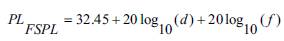
Path Loss in Free Space PLFSPL defines how much strength of the signal is lost during propagation from transmitter to receiver. FSPL is diverse on frequency and distance. The calculation is done by using the following equation [3]:

Here, f=frequency [MHZ],

d= distance between transmitter and receiver

1.2 Cost 231 HataModel

The basic path loss equation for this COST-231 Hata Model can be expressed as [4]:

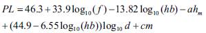
Where, d: Distance between transmitter and receiver antenna [km]

f: Frequency [MHZ]

h_b : Transmitter antenna height [m]

The parameter cm has different values for different environments like 0 dB for suburban and 3 dB for urban areas and the remaining parameter  a_hm is defined in urban areas as

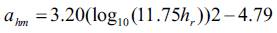
for f > 400MHz

The value for (a_hm ) in suburban and rural (flat) areas is given as

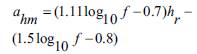
Where, hr is the receiver antenna height in meter.

1.3 Stanford University Interim (SUI) Model

The basic path loss expression of The SUI model with correction factors is presented as [4]

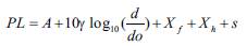
for, d > d_o

Where the parameters are

d: Distance between BS and receiving antenna [m]

d_o : 100 [m]

λ: Wavelength [m]

X_f: Correction for frequency above 2 GHz [MHZ]

X_h: Correction for receiving antenna height [m]

S: Correction for shadowing [dB]

γ(gama): Path loss exponent

The random variables are taken through a statistical procedure as the path loss exponent γ and the weak fading standard deviation s is defined.

The log normally distributed factor s, for shadow fading because of trees and other clutter on a propagation path and its value is between 8.2 dB and 10.6 dB [6].

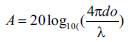
The parameter A is defined as

and the path loss exponent γ is given by

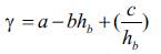
Where, the parameter h_b is the base station antenna height in meters. This is between 10 m and 80 m. The constants a, b and c depend upon the types of terrain, that are given in Table 1. The value of parameter γ = 2 for free space propagation in an urban area, 3 < γ < 5 for urban NLOS environment, and γ> 5 for indoor propagation.

The frequency correction factor X_f and the correction for receiver antenna height X_h for the models are expressed in:

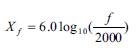
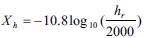for Terrain Type A and B

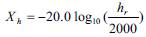for Terrain Type C

Where, f is the operating frequency in MHz, and h_r is the  receiver antenna height in meter. For the above correction factors this model is extensively used for the path loss prediction of all three types of terrain in rural, urban and suburban environments.

1.4 Ericsson Mod

Path loss according to this model is given by [5]:

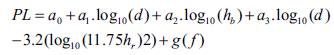
Where g (f) is defined by:

f : Frequency [MHZ]

h_b: Transmission antenna height [m]

h_r: Receiver antenna height [m]

The default values of these parameters (a₀ , a₁ , a₂ and a₃ ) for different terrain are given in Table 2:

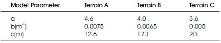
Table 1. Types of Terrain

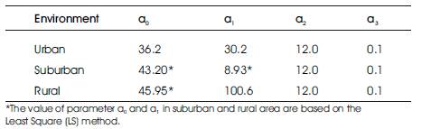
Table 2. Default values of parameters for different terrain

2.1 Path Loss in Urban Area for Fixed WiMAX

In calculation, they set 3 different antenna heights (i.e. 9 m, 12 m and 16 m) for receiver, distance varies from 250 m to 5 km and transmitter antenna height is 30 m. The numerical results for different models in urban area for different receiver antenna heights are shown in the Figures 1to3 (Table 3).

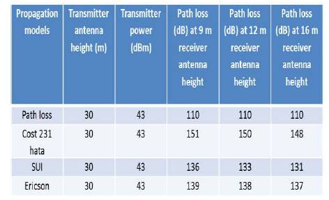
Table 3. Path loss estimate at 2 km distance in urban environment

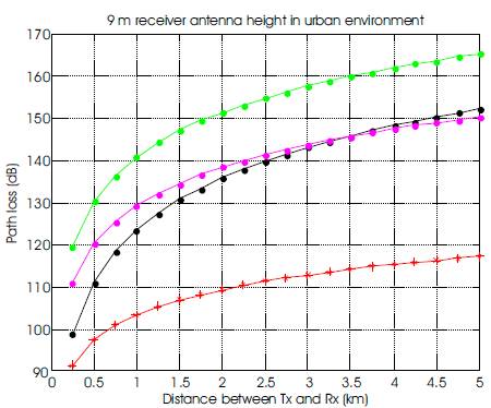
Figure 1. Path loss in urban environment at 9 m receiver antenna height

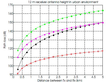
Figure 2. Path loss in urban environment at 12 m receiver antenna height

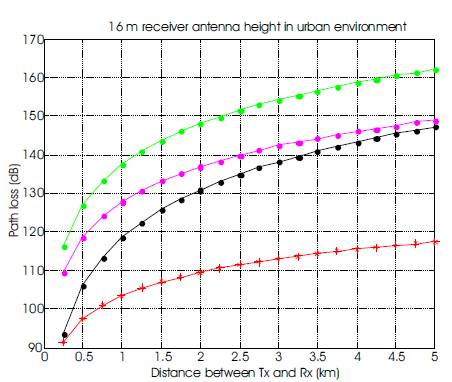
Figure 3. Path loss in urban environment at 16 m receiver antenna height

2.2 Path loss in suburban area for Fixed WiMAX

The transmitter and receiver antenna heights are same as used earlier. The numerical results for different models in suburban area for different receiver antenna heights are shown in Figures 4 to 6 (Table 4).

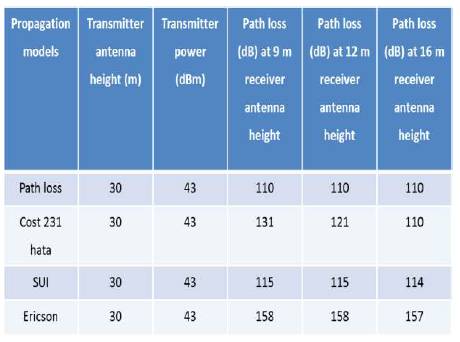
Table 4. Path loss estimate at 2 km distance in suburban environment

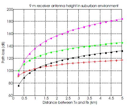
Figure 4. Path loss in suburban environment at 9 m receiver antenna height

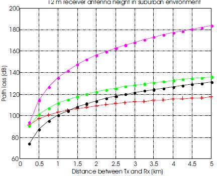
Figure 5. Path loss in suburban environment at 12 m receiver antenna height

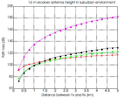
Figure 6. Path loss in suburban environment at 16 m receiver antenna height

2.3 Path loss in rural area for Fixed WiMAX

The receiver antenna heights are same as used earlier. Here the authors considered 20 m for transmitter antenna height. The numerical results for different models in rural area for different receiver antenna heights are shown in Figures 7-9 (Table 5).

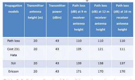
Table 5. Path loss estimate at 2 km distance in rural environment

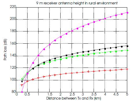
Figure 7. Path loss in rural environment at 9 m receiver antenna height

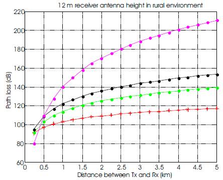
Figure 8. Path loss in rural environment at 12 m receiver antenna height

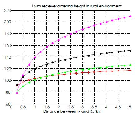
Figure 9. Path loss in rural environment at 16 m receiver antenna height

2.4 Path Loss in Urban Area for Mobile WiMAX

In calculation, they set 3 different antenna heights (i.e. 9 m, 12 m and 16 m) for receiver, distance varies from 230 m to 2 km and transmitter antenna height is 30 m. The numerical results for different models in urban area for different receiver antenna heights are shown in the Figures 10 to12 (Table 6).

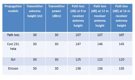
Table 6. Path loss estimate at 1 km distance in urban environment

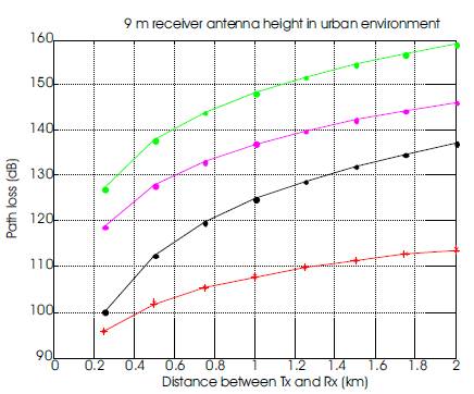
Figure 10. Path loss in urban environment at 9 m receiver antenna height

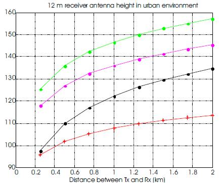
Figure 11. Path loss in urban environment at 12 m receiver antenna height

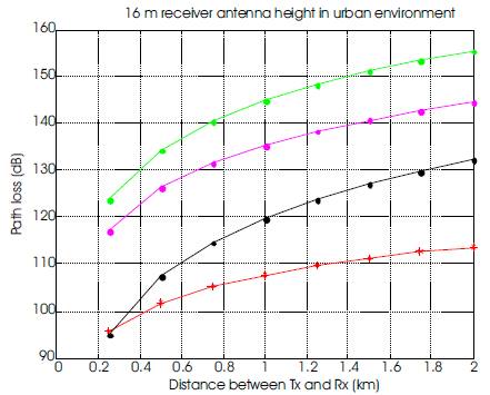
Figure 12. Path loss in urban environment at 16 m receiver antenna height

2.5 Path loss in suburban area for Mobile WiMAX

The transmitter and receiver antenna heights are same as used earlier. The numerical results for different models in suburban area for different receiver antenna heights are shown in the Figures 13-15 (Table 7).

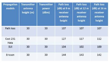
Table 7. Path loss estimate at 1 km distance in suburban environment

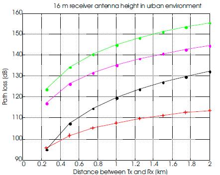
Figure 13. Path loss in suburban environment at 9 m receiver antenna height

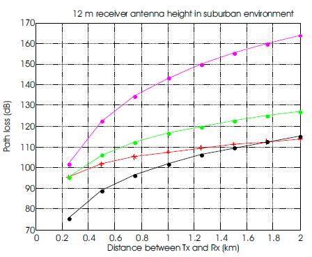
Figure 14. Path loss in suburban environment at 12 m receiver antenna height

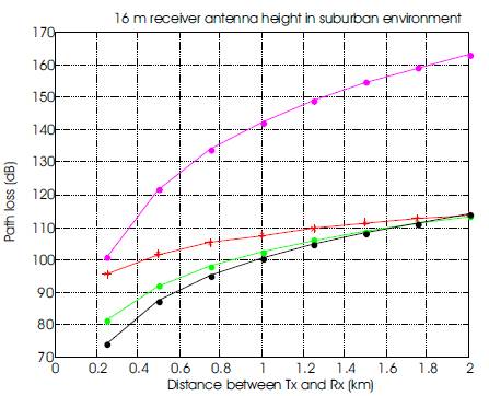
Figure 15. Path loss in suburban environment at 16 m receiver antenna height

2.6 Path loss in rural area for Mobile WiMAX

The receiver antenna heights are same as used earlier. Here they consider 20 m for transmitter antenna height. The numerical results for different models in rural area for different receiver antenna heights (Figures 16-18)(Table 8).

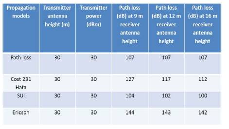
Table 8. Path loss estimate at 1 km distance in rural environment

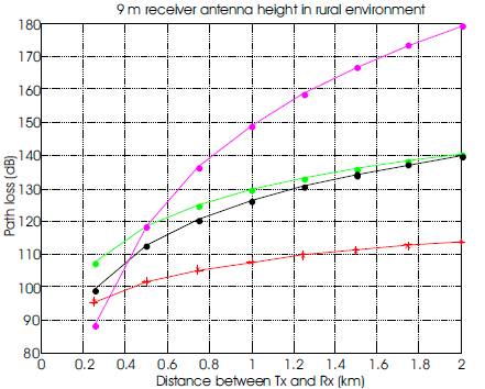
Figure 16. Path loss in rural environment at 9 m receiver antenna height

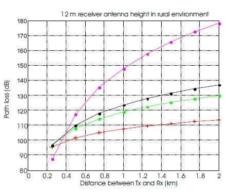
Figure 17. Path loss in rural environment at 12 m receiver antenna height

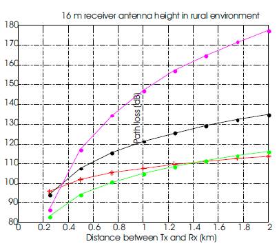
Figure 18. Path loss in rural environment at 16 m receiver antenna height

After simulating the following comparisons can be made based on the Figures 19 to 24 and Tables 9 to 14. All the comparisons are done with three WiMax environments (Urban, suburban and rural) in Fixed and Mobile WiMax systems.

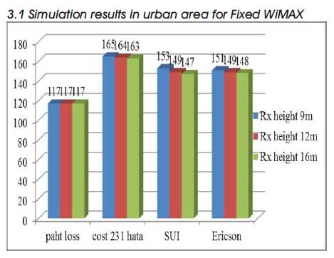
Figure 19. Analysis of simulation results for urban environment in different receiver antenna height

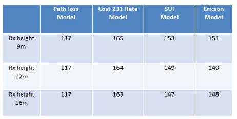
Table 9. Analysis of simulation results for urban area in different receiver antenna height(distance 5km)

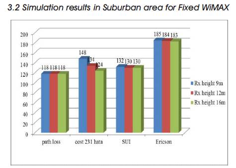
Figure 20. Analysis of simulation results for Suburban environment in different receiver antenna height.

Table 10. Analysis of simulation results for Suburban area in different receiver antenna height (distance 5km)

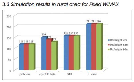
Figure 21. Analysis of simulation results for rural environment in different receiver antenna height.

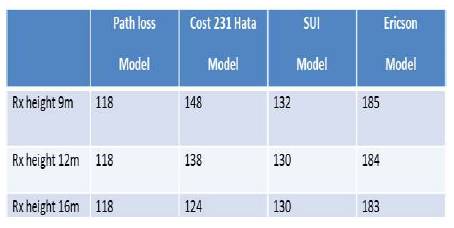
Table 11. Analysis of simulation results for rural area in different receiver antenna height (distance 5km)

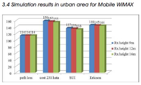
Figure 22. Analysis of simulation results for urban environmentin different receiver antenna height.

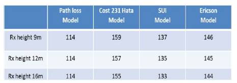
Table 12: Analysis of simulation results for urban area in different receiver antenna height (distance 5km)

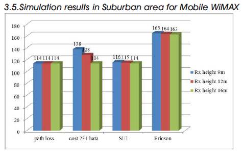
Figure 23. Analysis of simulation results for suburban environment in different receiver antenna height.

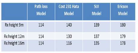
Table 13. Analysis of simulation results for suburban area in different receiver antenna height (distance 5km)

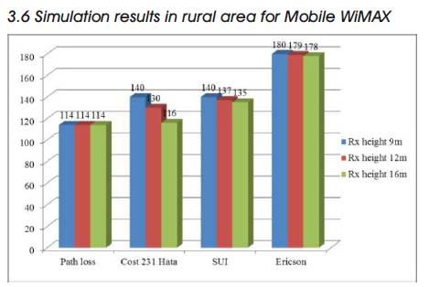
Figure 24. Analysis of simulation results for rural environment in different receiver antenna height.

Table 14. Analysis of simulation results for rural area in different receiver antenna height (distance 5km)

After all condition they applied and the result they got we can calculate the work as they studied WiMAX standards, Modulation Techniques, WiMAX Network Architecture Model, and Mobility System with the help of proper figure. We studied Cost- 231 Hata, Ericsson and SUI Model and implemented it through MATLAB simulation to evaluate the Network Performance at urban, sub-urban and in rural area by Path-Loss calculation. The authors also used and understood different antenna height technique at different environment for measuring the Network Performance.

From the result we see that, Ericsson model showed the lowest and Cost-231 Hata model showed the highest Path- Loss for fixed WiMAX in urban area where, for mobile WiMAX SUI model showed the lowest and Cost-231 Hata predict highest Path-Loss in this environment. In sub-urban area, SUI model showed the lowest and Ericsson showed the highest Path-Loss for Fixed WiMAX, where for mobile WiMAX SUI model showed the lowest and Ericsson model showed highest Path-Loss in this environment. In rural, Cost-231 Hata showed the lowest and Ericsson showed highest Path-Loss for Fixed WiMAX, where for mobile WiMAX Cost-231 Hata showed lowest and Ericsson showed highest Path-Loss in this environment. Their comparative analysis indicates that they did not find any single model that can be recommended for all environments.

In case of antenna technique, the authors see that whenever they increase the distance between Tx and Rx Path-Loss also increase and when the consider high receiver antenna they found Path-Loss is lower compared to lower receiver antenna for fixed and mobile WiMAX.

Finally we can conclude that fixed and mobile WiMAX both have some advantages and disadvantages. Fixed WiMAX can give high data rate to a user but can't give mobility at vehicular speed, where mobile WiMAX can give mobility at vehicular speed but data rate is slower compared to fixed WiMAX. Though mobile WiMAX can give high data rate if it got higher frequency and closer adjacent cell but then cost will be high.