Figure 1. Create or Open Project
Slopes are either man-made (cuttings, embankments for highways, railroads, etc.) or natural (hillside, valleys). Slopes are of two types, viz., finite and infinite. Forces due to instability are force of gravity, force of seepage, earthquake forces, etc. (Ranjan and Rao, 2007). Slope failures are of two types, viz., translational and rotational. Slopes can be analysed by many methods, such as Total stress analysis, Swedish circle method or Method of slices, Bishop's method, Friction circle method, Stability number method, etc. Other than these, different types of software are available for analysis in stability of slopes, for eg: Geoslope, Visual Slope, Geo- Techpidia, C programming, etc. The present work is to analyse the stability of slopes using Visual Slope. Visual Slope is a user-friendly software used for analysis in stability of slopes. By calculating the different input parameters for different trials, least Factor of Safety (F.O.S) could be obtained so that slope can be analysed and stabilised. By using this software, large amount of arithmetic operations can be done within in a few seconds and hence very useful to engineers in the analysis of slope stability.
Slopes are artificial or man-made cuttings and embankments for highways and railroads (Visual Slope User's Guide Version 6, 2016), Natural-hillsides, and valleys. Forces which cause instability are force of gravity, force of seepage, earthquake forces, etc.
Infinite slopes: Slope of a semi-infinite soil mass is an infinite slope, where the soil properties below surface are constant (Visual Slope, n.d.).
Finite slopes: Slope length is limited in finite slopes. Eg: earthen dams, cuts, etc.
Translational Failure: Failures occur along a long surface parallel to slope at some depth.
Rotational Failure: Failures occur by rotation along slip surface (Punmia and Jain, 2005).
Methods to analyse finite slopes:
Software, such as Geoslope, Visual Slope, Geo Techpedia, C programs, etc., are available for the analysis in stability of slopes. The study is to analyse stability of slopes using Visual Slope and C program. By calculating different input parameters for different trials, the least Factor of Safety (FOS) was found finally so that slope can be analysed and stabilised (Geotechpedia, n.d).
Visual slope is a user-friendly software used in analysis of stability of slopes (Visual Slope, n.d.).
By using this software, large amount of arithmetic operations can be done within a few seconds. So, it is very useful to engineers in the analysis of slope stability (Oasys, 2018). Uncertainties about the geometry of the slope and the properties of the various soils within the slope can be investigated in detail. Many trial failure surfaces can be analysed. More accurate methods that satisfy statics can be used (China Knowledge Network, n.d.).
It is a multi-function engineering computer program developed for:
All functions are in series as follows:
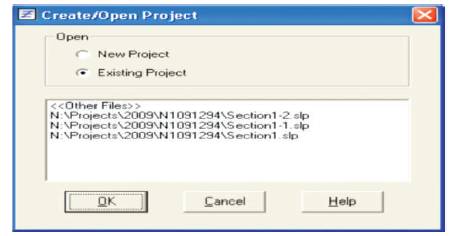
Figure 1 shows that the user chooses either a new project or an existing project, and can able to change the settings later also by selecting general settings as shown in Figure 2 and the settings are displayed in Figure 3.
Figure 1. Create or Open Project
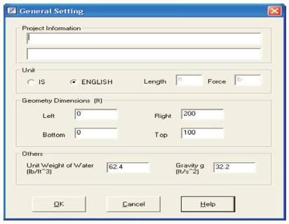
Figure 2. General Settings
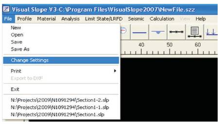
Figure 3. Change Settings
Software consists of different types of lines, such as Soil lines, Georgid lines, Water table lines, etc., as shown in Figure 4. Line buttons are used to draw different lines as shown in Figure 5.
When a correct line type is chosen, the user can draw the line and can begin to draw a profile. Two methods to draw a line are as follows.
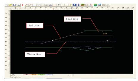
Figure 4. Visual Slope Profile
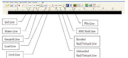
Figure 5. Line Buttons
Figure 4 represents that line can be drawn and the type of line can be chosen as shown in Figure 5.
Right clicking or using escape button can stop drawing line.
Figure 6 shows the coordinate indicators that can be selected and used in horizontal and vertical coordinates into box as shown in Figure 7 and enter key is pressed and then line will get started. Same method is used for end point also. It can also use length and angle method as shown in Figure 8.
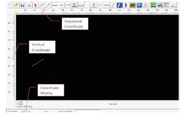
Figure 6. Coordinate Indicators
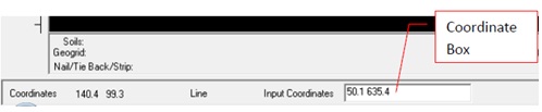
Figure 7. Coordinate Input
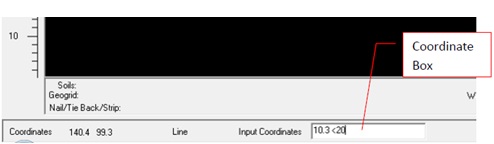
Figure 8. Lenth-Angle Input
If any points of old and new lines match the feature, it shows either Delete or Editing of Line.
Select the line to be deleted as shown in Figure 9. Click delete button to get the line deleted.
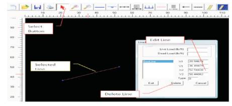
Figure 9. Delete or Editing of Line
As shown in Figure 10, click on load button and draw surcharge load from left to right. Initial load intensity is 1. To change this, line edit method was used. User should specify live or dead load.
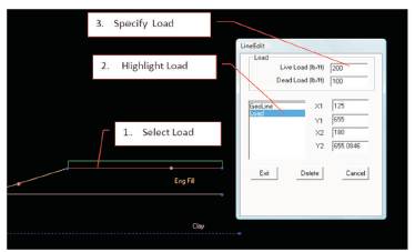
Figure 10. Adding Surcharge Load
The other features available, such as Zoom in, Zoom out, Undo, Flip, and PDF are as shown in Figure 11.
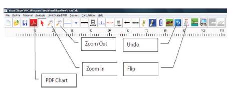
Figure 11. All other Features
They include,
Bank is available for most used properties and able to select from them.
Sotware can perform into three types of slope stability analysis.
The three types can also be analysed using Spencer's method.
From analysis menu, circular failure is chosen as shown in Figure 12. Input box of circular failure appear as shown in Figure 13. Circular failure can be specified using 5 numbers:
Coordinates can be typed in dialogue box as shown in Figure 13.
Number of failure surfaces should be at least 500 and should be an integer, where Spencer method can also be used after entering data click calculation button for analysis. To see failure surfaces, click on curve button as shown in Figure 14.
The software has other features, such as
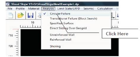
Figure 12. Analysis of Circular Failure
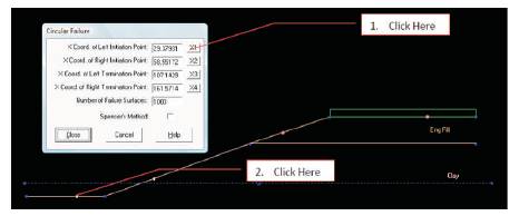
Figure 13. Circular Failure Analysis Setup
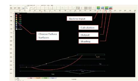
Figure 14. Analysis Result
Profile for the slope: Slope profile can be established as shown in Figure 15 and Coordinate points are shown in Figure 16.
Figures 17 and 18 show the 6 most and 500 critical surfaces.
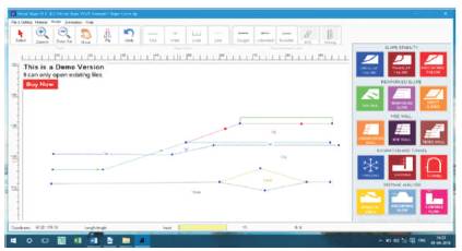
Figure 15. Slope Profile
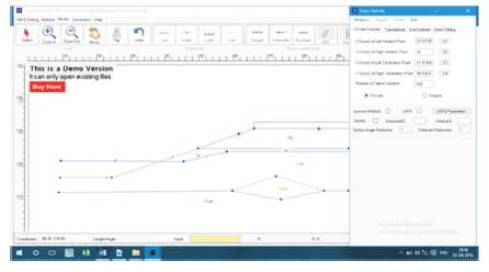
Figure 16. Figure Showing Coordinate Points
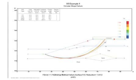
Figure 17. 6 Most Critical Failure Surfaces for Circular Case

Figure 18. 500 Failure Surfaces for Circular Case
Figures 19 and 20 show the 6 most and 500 critical surfaces.
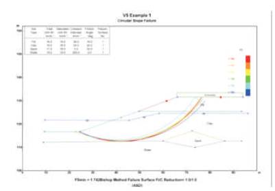
Figure 19. 6 Most Critical Failure Surfaces for Seismic Analysis
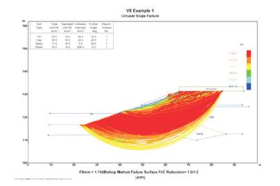
Figure 20. 500 Failure Surfaces for Seismic Analysis
LRFD parameters: Parameters to be considered in LRFD check are shown in Figure 21. Figures 22 and 23 show the 6 most and 500 critical surfaces.
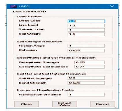
Figure 21. LRFD Parameters
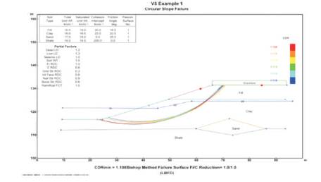
Figure 22. 6 Most Critical Failure Surfaces for Limit State Method
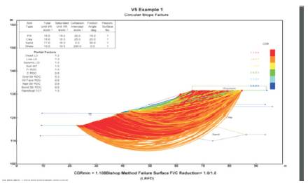
Figure 23. 500 Failure Surfaces for Limit State Method
Figures 24 and 25 show the 6 most and 500 critical surfaces.
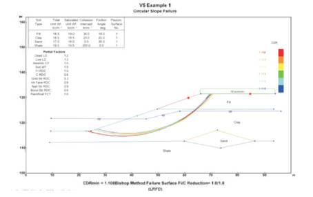
Figure 24. 6 Most Critical Failure Surfaces for LRFD and Seismic Case
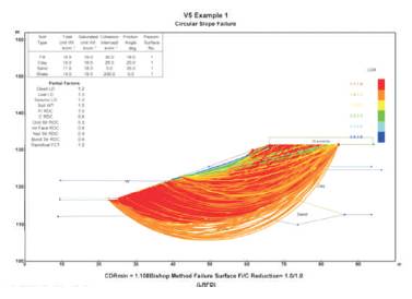
Figure 25. 500 Failure Surfaces for LRFD and Seismic Case
Figures 26 and 27 show the 6 most and 500 critical surfaces.
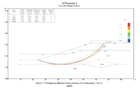
Figure 26. 6 Most Critical Failure Surfaces for Spencer’s Method
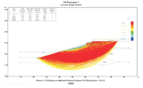
Figure 27. 500 Failure Surfaces for Spencer’s Method
Figures 28 and 29 show the 6 most and 500 critical surfaces.
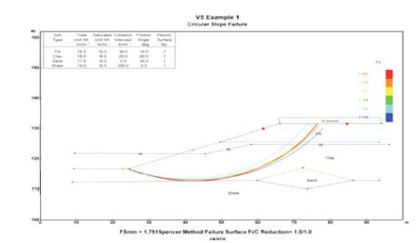
Figure 28. 6 Most Critical Failure Surfaces for Spencer’s and Seismic
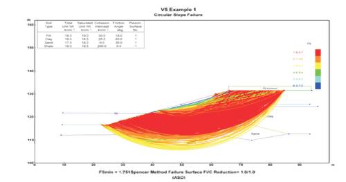
Figure 29. 500 Failure Surfaces for Spencer’s and Seismic
Figures 30 and 31 show the 6 most and 500 critical surfaces.
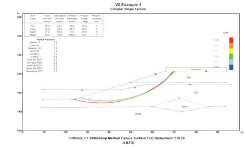
Figure 30. 6 Most Critical Failure Surfaces for Spencer’s and LRFD
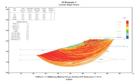
Figure 31. 500 Failure Surfaces for Spencer’s and LRFD
Figure 32 and 33 show the 6 most and 500 critical surfaces.
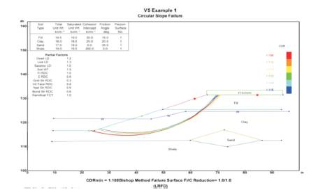
Figure 32. 6 Most Critical Failure Surfaces for Spencer’s Case

Figure 33. 500 Failure Surfaces for Spencer’s Case
Figures 34 and 35 show the 6 most and 500 critical surfaces.
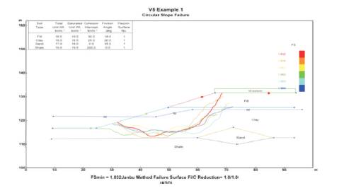
Figure 34. 6 Most Critical Failure Surfaces for Irregular Failure
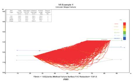
Figure 35. 500 Failure Surfaces for Irregular Failure
Figures 36 and 37 show the 6 most and 500 critical surfaces.
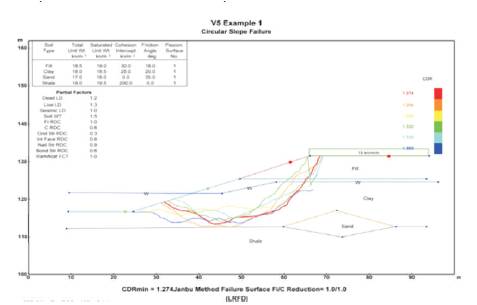
Figure 36. 6 Most Critical Failure Surfaces for Irregular and LRFD
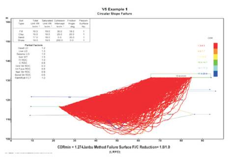
Figure 37. 500 Failure Surfaces for Irregular and LRFD
Figures 38 and 39 show the 6 most and 500 critical surfaces.
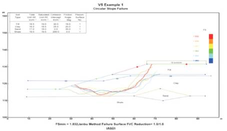
Figure 38. 6 Most Critical Failure Surfaces for Irregular and Seismic
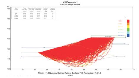
Figure 39. 500 Failure Surfaces for Irregular and Seismic
Figure 40 and 41 show the 6 most and 500 critical surfaces.
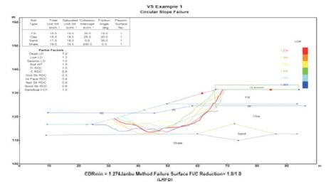
Figure 40. 6 Most Critical Failure Surfaces for Irregular Case
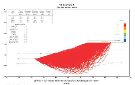
Figure 41. 500 Failure Surfaces for Irregular Case
In Spencers method it is not possible.
In Modified Bishop Method, least FOS is 1.742 and seismic also remains the same because horizontal and vertical accelerations are taken as 0, 0. Even if there is increase in FOS, it also increases to hundreds and if there is a reduce, it decreases to a negative value. By appling limit state or LRFD parameters, FOS can be reduced to 1.108. Comparatively limit state method gives least FOS as shown in Table 1.
In Spencer's method least FOS is 1.751 and after applying seismic loads, FOS is 1.680. By applying limit state method or LRFD parameters, FOS can be reduced to 1.108. Comparitively limit state method gives least FOS as shown in Table 2.
In Janbu method, least FOS is 1.832 and seismic also remained the same. By applying limit state or LRFD parameters, FOS is reduced to 1.274. Comparivitely LRFD gives least FOS as shown in Table 3.
In Spencer's method, it is not possible because spencers method requires radius for calculation of FOS. But in irregular failure, there is no radius.
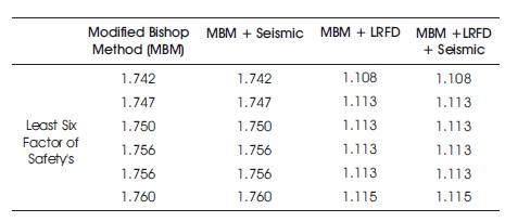
Table 1. Comparison of FOS with Different Approaches (Modified Bishop Method)
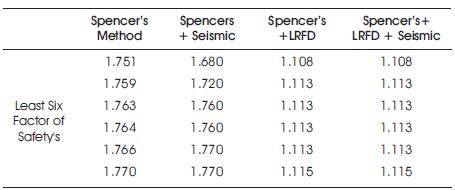
Table 2. Comparision of FOS with different Approaches(Spencer's Method)
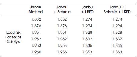
Table 3. Comparision of FOS with Different Approaches(Janbu Method)
In recent times, computer applications are widely used in geotechnical studies. Analysing slope stability can be done in a more advanced way. Hence this study is very useful in such cases by utilising Visual Slope and C programming. In Visual slope Circular failure, the least FOS is obtained as 1.108 and in irregular failure, it is 1.274.