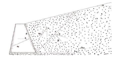
Figure 1. Forces Acting on a Retaining Wall
This paper presents the comparison of the various methods of analysis of retaining walls under seismic loads. The furthermost usually used methods for the seismic design of retaining walls were considered. A concrete retaining wall was considered and analyzed for the static as well as the seismic loading conditions. It is formed that internal friction angle and soil-wall friction angle affect the stability on the basis of parametric studies. The authors have calculated the factor of safety against sliding and overturning. Two Statics and four dynamic methods for zone four (IV) have been studied and compared for their factor of safety. Amongst the six methods being studied, Choudhury and Nimbalkar [ 3] came out for maximum factor of safety. Whereas Seed and Whitman [ 12] with minimum factor of safety. Hence the method used by Choudhury and Nimbalkar is recommended for earthquake prone areas on the basis of this study. It is also found that Seed and Whitman (1970) are more conservative as compared to other methods.
Earthquake resistant strategies of soil retaining constructions like retaining walls, earth dams [1], foundations are actually significant towards reducing the shocking consequence of seismic exposures. The Retaining wall is an arrangement whose principal objective is toward inhibiting side movement. The pressure and forces on the walls of an amount of venerated wall-soil glitches are evaluated. The enlightenments acquired are estimated for an assortment of the significant parameters to give results valuable for design [14]. Seismic solidity of earth retaining structures [14] remains usually as an analysis by Pseudo-static methodology in which properties of earthquake forces are expressed in the form of straight and perpendicular accelerations [4]. The study of seismic dynamic ground pressure is necessarily aimed at the not dangerous strategy of retaining wall in the Seismic region. Various scientists obligate established numerous approaches to control the seismic dynamic soil pressure on an inflexible retaining wall owing to earthquake stuffing original stuffingoriginal work on earthquake-induced horizontal earth pressure below dynamic and passive circumstances acting on a retaining wall [5]. The static soil pressures on retaining buildings are muscularly predisposed by wall and earth activities. The dynamic soil pressures grow by retaining wall changes absent from the soil behind the situation, including extensional horizontal pressure cuttingedge of the earth. Subsequently the wall association remains sufficient near activated asset of the earth after the wall and least active soil pressures act preceding the wall. For actual tiny wall association be situated, it is obligatory to grow least dynamic soil pressures (aimed at the normal situation of cohesion-less backfill resources), allowed standing retaining walls be situated typically deliberate happening on the basis of least dynamic soil pressures, wherever horizontal wall activities are controlled, such by way of in the cases of tie-back walls, fastened bulkheads, cellar walls, passage struts, immobile soil pressures could remain superior to least dynamic. Passive ground pressures grow equally a retaining wall transfer to the earth, generating compressive horizontal straining in the earth.
After the strong point of the earth is completely mobilized, extreme passive soil pressures performance happens. Constancy of numerous free-standing retaining walls is contingent retaining the equilibrium amongst dynamic pressures temporary predominantly proceeding unique cross off the wall and then inactive pressures act proceeding the additional. Soil retaining buildings, such by way of retaining walls, passage struts, dockside parapets, and fastened bulk crowns, fixed diggings also routinely steadied walls, are used all over seismically dynamic zones. Commonly signify vital fundamentals of harbors and ports, conveyance system, links and additional assembled conveniences. Earthquakes have produced stable deformation of retaining buildings in numerous past earthquakes. In many cases, these distortions are there in negligible minor. In others, they formed significance destruction. In nearly circumstances, retaining structures must distort throughout earthquakes, by devastating somatic and financial significances. This study presents the role of various soil parameters in the design of retaining wall [3].
The seismic behaviour [7] of retaining walls is governed by the entire horizontal soil pressures that grow throughout earthquake trembling. The entire weights comprise equally the stationary gravitational pressures that exist previously as the occurrence of an earthquake and temporary dynamic pressures induced by the earthquake. Figure 1 illustrates the various factors performing on a retaining wall underneath stationary loading.
Figure 1. Forces Acting on a Retaining Wall
Uniform under-stationary circumstances, forecast real retaining walls forces plus distortions remain difficult making earth structure collaboration a problematic one. Distortions remain frequently in the considered new design. The characteristic method is toward approximation of the forces performing, preceding a wall and then to strategy the wall toward counter attack of individuals forces using a factor of safety great sufficient to create adequately minor distortions. A number of basic methods is obtainable to assess stationary loads on retaining walls [9]. Utmost usually used are labelled in the subsequent segments .
There have been many approaches adopted in the recent times depending upon the forces acting and the displacement occurred during a seismic activity, which are as follows.
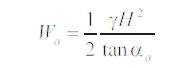
A retaining wall is considered as shown in Figure 2 with height 4 m and considered as thickness of the reinforced concrete wall stem as 0.4 m. The reinforced concrete wall footing is 3 m wide by 0.5 m thick. The unit weight of concrete is taken as 23.50 kN/m3 . The wall backfill consists of sand having Φ =32° (degree) and γ1=20 kN/m3 (unit weigh of soil). The friction angle between the bottom of the footing and the bearing soil was taken as δ =38°. Some values are given following parameters -Wa = 907.40509 kN, Wp = 1215.320658 kN, Q ha= 1306, Qva =695, Qhp = 489, Qvp =438, αa= 10, αp=7.5, Φ= 32, ψ= 15. Assumed that the wall lies in the earthquake zone four (IV) of India. It is with seismic coefficient KhE = 0.36.
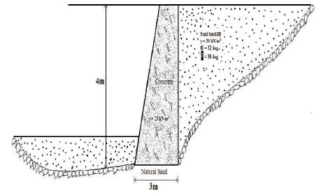
Figure 2. Sketch of Typical Retaining Wall
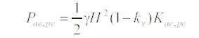
a) Active Earth Pressure:
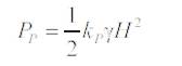
b) Passive Earth Pressure:
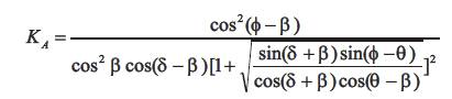
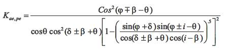
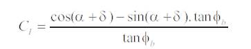
a) Active Earth Pressure Coefficient:
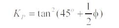
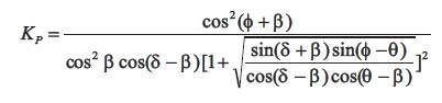
b) Passive earth pressure coefficient:
2.2.1 Pseudo Static Method: (Mononobe - Okabe Method) [8] [10]
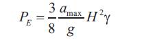
2.2.2 Seed and Whitman Method [11] [12]:-

2.2.3 Richards-Elms Method
a) Dynamic Condition:
b) Statics Condition:
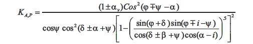
2.2.4 Choudhury & Nimbalkar [2] [3]:-
a) Seismic Active Earth Pressure:
b) Seismic Passive Earth Pressure:
The effect of internal friction angle (Ф) with the different methods used above in the graph. The variation of internal friction angle (Ф) with respect to active earth pressure coefficient (ka ), all the method variation is approximately linear, but in Mononobe-Okabe (1929, 1926) [8], [ 10], the variation is highly increased. In all the methods, the internal friction angle (Ф) is inversely proportional to active earth pressure coefficient (ka ) as in Figure 3.
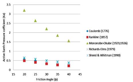
Figure 3. The Variation of Active Earth Pressure Coefficient (ka ) with Internal Friction Angle (Φ)
The effect of internal friction angle (Ф) with the different method used in the graph. The variation of internal friction angle (Ф) with respect to passive earth pressure coefficient (ka), all the method variations are approximately linear, but in Coulomb (1776) the variation in highly increased. In all the methods, the internal friction angle (Ф) is directly proportional to passive earth pressure coefficient (kp) in Figure 4.
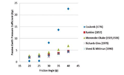
Figure 4. The Variation of Passive Earth Pressure Coefficient (kp ) with Internal Friction Angle (Φ)
The effect of internal friction angle (Ф) with different methods used is shown in the graph. The variation of internal friction angle (Ф) with respect to active earth pressure (Pa), all the method variations are approximately linear, but in Mononobe-Okabe (1929, 1926) and Choudhury and Nimbalkar, the variation is highly increased. In all the methods, the internal friction angle (Ф) is inversely proportional to active earth pressure (Pa) in Figure 5. If the internal friction angles are increased, the active earth pressure is decreased and vice versa.
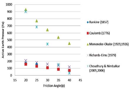
Figure 5. The Variation of Active Earth Pressure (ka) with Internal Friction Angle (Φ)
The effect of internal friction angle (Ф) with the different methods used above in the graph. The variation of internal friction angle (Ф) with respect to passive earth pressure (Pp), all the method variations are approximately linear, but in Coulomb (1776) the variation is highly increased. In all the methods, the internal friction angle (Ф) is directly proportional to passive earth pressure (Pp) as in Figure 6. If the internal friction angles are increased then the passive earth pressure is increased and vice versa.
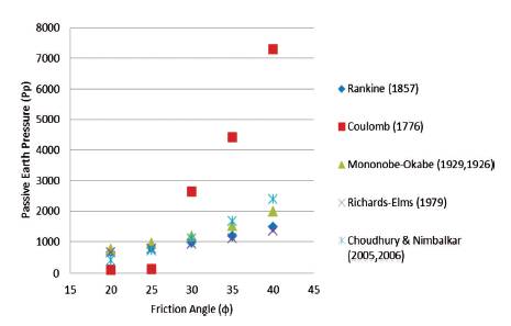
Figure 6. The Variation of Passive Earth Pressure (Pp) with Internal Friction Angle (Φ)
As can be noted from the graphical representations of the results obtained from the application of different theories, the active earth pressures coefficients is not strongly affected by the soil wall friction angle δ, while minor variations of δ produce great differences in KP values calculated by various methods.
From Figures 1 to 4, the comparisons between the normal components to the wall of the active and passive earth pressure coefficients evaluated with the different methods for a horizontal backfill ( ε=0) retained by smooth ( δ=0) and rough( δ= φ) vertical walls are plotted. Note that the earth pressure coefficients was estimated till to a soil friction angle φ=40°. The passive earth pressure coefficients are more sensible to the soil wall friction. If the log spiral method can be interpreted as the most accurate determination close to the exact solution, the Coulomb method provides KP values very similar to those expected while Rankine method gives conservative and easy-to-calculate passive coefficients.
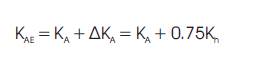
For the active case, the KAE values obtained by Seed-Whitman method and M-O methods are practically identical. This is due to the fact that, when the wall is almost vertical and the slope angle of the backfill is bigger than zero, the most critical failure is practically planar.
In the passive case, the most critical sliding surface is much different from a planar surface as is assumed in the M-O analysis. The KPE values are seriously overestimated by the M-O method. They are, in most cases, higher than those obtained from Seed-Whitman. This is especially the case when the wall is rough and the angle of wall repose is large. The condition φ= δ= 40° carries out very high KPE values larger than 20, unreported in figures. For smooth walls, the potential sliding surface is practically planar and the different methods give almost identical results.
The other two seismic methods are Richards-Elms and Choudhury & Nimbalkar calculated the Factor of safety with different parameters.
The values of factor of safety for sliding and overturning from the static and seismic analysis using KhE = 0.36 (Zone the four) are briefed below in Table 1.
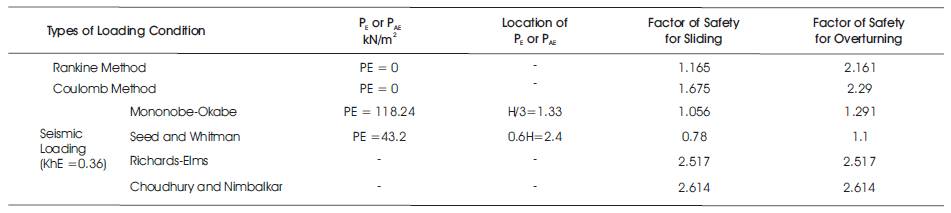
Table 1. Factor of Safety for Sliding and Overturning by Different Methods
For the analysis of sliding and overturning of the retaining wall, it is common to accept a lower factor of safety (1.10 to 2.20) under the combined static (stationary) and earthquake (dynamic) loads. It is evident from Table 1 that Seed & Whitman method (1970) gives lesser value of factor of safety as related to other methods considered in this study. Thus, it is a recommended (suggested) method for the design of retaining walls in earthquake (trembling) prone region.
It has been observed by parametric study that active earth pressure coefficient are almost identical by different methods, it can be noted from the graphical representations of the results obtained from the application of the different theories, the active earth pressures coefficients is not strongly affected by the soil wall friction angle δ, while, small variations of δ produce large differences in KP values calculated by various methods.
1. Rankine Method [4]:
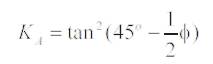
Ka = tan2 (45o - 1/2 Φ) = 0.307 by using equation (2)
Kp = tan2 (45o + 1/2Φ ) = 3.25 by using equation (4)
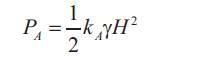
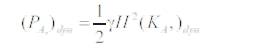
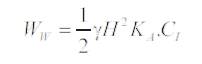
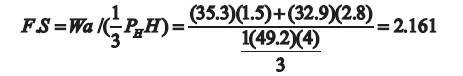
(PA) = 1/2 kAγtH2= (0.5)*(0.307)*(20)*(42) = 49.2 kN/m by using equation (1)
(Pp) = 1/2 kpγtD2 = (0.5)*(3.25)*(20)*(0.52 ) = 8.14 kN/m by using equation (3)
By applying reduction factor =1.99 = 2,
Pp = 4.067kN/m
Footing Weight = (3)* (0.5) *(23.5) = 35.301kN/m
Stem Weight = (0.4)* (3.5)* (23.5) = 32.901kN/m
N = Weight of concrete wall = 35.3 + 32.9 = 68.20 kN/m
By taking moments about the toe of the wall to determine location of N,
Nx=-PA (4/3)+W(moment arms) ….This gives X = 1.1645 m
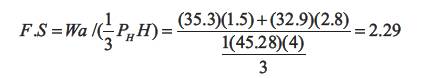
Factor of safety for sliding: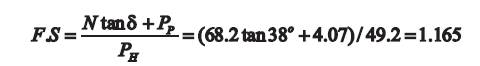
Factor of safety for overturning:
2. Coulomb Method:
KA = 0.283 by using equation (5)
KP = 21.7 by using equation (6)
(PA ) = 1/2 kAγtH2 = (0.5)*(0.283)*(20)*(42) = 45.28 kN/m by equation (1)
(PP ) = 1/2 kpγtD2 = (0.5)*(21.7)*(20)*(0.52) = 54.25 kN/m by equation (3)
By applying reduction factor = 2,
Pp = 27.125kN/m
Footing Weight = (3)*(0.5)*(23.5) = 35.301kN/m
Stem Weight = (0.4)*(3.5)*(23.5) = 32.901 kN/m
N = Weight of concrete wall = 35.3 + 32.9 = 68.20 kN/m
By taking moments about the toe axis of the wall to determine location of N,
Nx=-PA (4/3)+W (moment arms) …. This gives x= 1.165m
Factor of safety for sliding: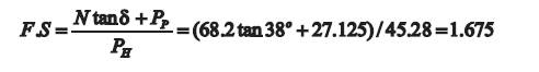
Factor of safety for overturning:
3. Seismic Analysis:
1. Pseudo Static Method (Mononobe-Okabe Method) [8] [10]:
KAE = 0.748 by using equation (8)
PAE = 117.24 kN/m by using equation (7)
Ψ= 19.78
Factor of safety for sliding = 1.056
Factor of safety for overturning = 1.291
4. Seed and Whitman Method [11], [12]:
PE = 43.2 kN/m by equation (9)
Factor of safety for sliding:
Factor of safety for overturning:
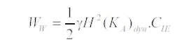
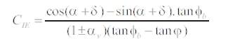
5. Richards – Elms Method:
After calculation-
(Ka )dyn =2839.48502 by using equation (13)
Ka =1794.831888 by using equation (13)
αv = .1
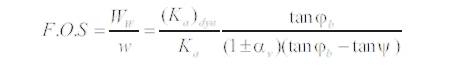
If, +ve sign then the F.O.S = 2.517
If, -ve sign then the F.O.S = 3.077
In comparison we take the value of +ve sign F.O.S.=2.517
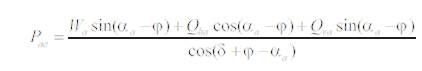
6. Choudhury & Nimbalkar[2] [3]:
After calculation –
Wa = 907.40509 kn by using equation (20)
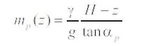
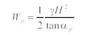
Wp = 1215.320658 kn by using equation (25)
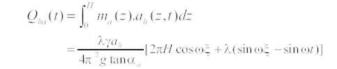
Qha = 1306 by using equation (21)
Qva =695 by using equation (22)
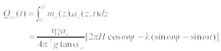
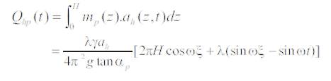
Qhp = 489 by using equation (26)
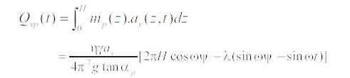
Qvp =438 by using equation (27))
αa=10 αp=7.5 Φ=32 Ψ=15
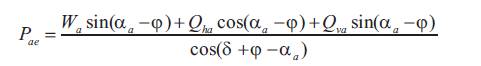
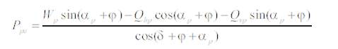
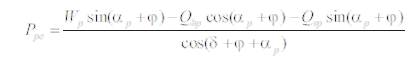
F.O.S =Pae/Ppe = 2.60
The authors have calculated the F.O.S. with the heap of different methods.