A Study on Parameters of Firefly Algorithm For Topology Optimisation of Continuum Structures – II
B. Archana * K.N.V. Chandrasekhar ** T. Muralidhara Rao ***
* M.Tech Student, Department of Civil Engineering, CVR College of Engineering, Hyderabad, Telangana, India.
** Assistant Professor, Department of Civil Engineering, CVR College of Engineering, Hyderabad, Telangana, India.
*** Professor & Head, Department of Civil Engineering, CVR College of Engineering, Hyderabad, Telangana, India.
Abstract
This paper is a continuation of the research work on Topology optimization of continuum structures using Firefly Algorithm. Tuning of parameters for meta-heuristic algorithms have been one of the emerging areas of research. The goal is to find a global minimum for an optimization problem in a d-dimensional space. Complex domains in structural engineering may require tuning of parameters to reduce the overall computational effort. In this paper, the main focus is on finding an optimum set of parameters required to perform topology optimization for a design domain. Few problems in the literature have been solved and the results were compared.
Keywords :
- Firefly,
- Meta-heuristics,
- Optimization,
- Parameters,
- Tuning,
- Continuum Structures.
Introduction
The swarm intelligence based algorithms [ 15], Cuckoo, Ant Colony, and Firefly algorithms have several advantages over the traditional algorithms. These meta-heuristics have been receiving considerable attention in the past three decades [ 8]. The simple fact is that meta-heuristics are good at continuous optimisation and are easier to implement as compared with the classical techniques, making them an ideal choice. The two main components of the meta-heuristic algorithms are intensification and diversification, popularly known as exploitation and exploration. They can generate diverse solutions simultaneously and explore the global search space effectively. One of the problems dealt in this paper will definitely strengthen this observation. Lin in his paper [ 6] made an attempt to the cantilever plate problem, which has been one of the difficult problems for quite some time in the literature. The search space is too narrow and the applied load is quite high. In this paper, the authors have made an attempt to identify two diverse material distributions, topologies for this cantilever plate problem which were not only clear and distinct, but also have lower weight in a fewer number of iterations. This is definitely an interesting and admiring ability of the Firefly meta-heuristic algorithm. Meta-heuristics usually require fewer parameters and the convergence rate is quite high. These metaheuristics algorithms start with an initial guess and converge toward a stable solution. The number of iterations required is relatively quite lower when compared with other algorithms. In this paper, the initial study has been performed using a few standard mathematical functions, Rastringin function, Rosenbrock, and Camel's back functions [ 8] have been thoroughly studied. These complex algorithms guarantee an optimal solution for NP Hard problems [ 8]. These require an exponential computational effort to arrive at the optimal solution.
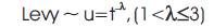
The Firefly algorithm has been widely used in structural optimisation over the last few years. The algorithm has been performing quite better when compared with the traditional Genetic algorithms and other meta-heuristic algorithms. The algorithm is a maximization algorithm which uses a few parameters, namely attractiveness parameter - beta, absorption coefficient - gamma, aggressiveness of random move - alpha, and levy distribution parameter - lambda [ 12]. Firstly, the authors present a brief overview of the parameters, what they mean and why they have to be used. A firefly's attractiveness coefficient is proportional to the light intensity as seen by other flies. The atmosphere surrounding the flies shall absorb the light proportional to the absorption coefficient denoted by gamma. A clear sky will have a lower value of absorption coefficient and thick foggy skies will have a higher value of the absorption coefficient. The value of absorption coefficient, gamma is input to the algorithm. When the value of gamma is nearly 1.0, the firefly algorithm tends to behave as a special case of Particle Swarm Optimisation (PSO) and when the value of absorption coefficient is very high, the flies cannot see each other and they tend to move randomly in space and hence the firefly algorithm behaves as a random algorithm. The fireflies shall follow a levy distribution having a thick fat tail when flies move towards each other. Another parameter, levy distribution parameter denoted by lambda decides the step length. The distance a fly can move towards another fly is known as step length. The direction is set by generating a random value between 0 and 1. When the random value is less than or equal to 0.5, it is taken as positive unity and when the random value is more than 0.5, the direction is taken as unity.
1. Aim of the Study
The purpose of this study is to find the optimum set of parameters for tuning the Firefly algorithm in order to optimize the optimization algorithm.
2. Objectives
The intended work is focused on optimizing a given continuum for a given material, loading and boundary conditions.
- To develop a new representation, wherein these representations of unstable and inefficient structures will actually point to stable configurations.
- To improve the efficiency of the optimisation process that uses an optimisation algorithm along with a proposed approach improves the input parameters to the optimization process.
3. Scope of the Study
The scope of the present study is as follows:
- Structures are assumed to be linear.
- Finite element analysis will not include the buckling analysis.
4. Methodology
Introducing a new mechanism, wherein these structures having disconnected regions and low stress regions can be removed and a structure with a stable configuration can be obtained. In other words, these unstable structures actually refer to a structure with a stable configuration and can compete with other fit individuals to explore the search domain and locate the optimal solution. As a result of this new representation schema, there will be more number of fit individuals exploring the search domain and also converge at a lower computational effort which forms the main objective of this study.
Literature review has been done extensively in this area of continuum optimization. The big challenge is to propose a new approach which will not only reduce the weight of the structure, but also in a fewer iterations at a lower computational effort. The proposed approach has been tested on several problems that are given in various journal papers and a few other textbooks. The study of the parameters involved tuning the optimization algorithm, in other words, optimizing the optimization algorithm and required lots of study. Several structures were optimized by varying the input parameters and the final converged optimized structure, a final optimum distribution of material within a given design domain is arrived at a lower computational effort.
5. Literature Review
Optimization is one of the oldest sciences that lead us further and mathematics is one of the ways to achieve the optimal state. The concept of optimization is basic too, much of what we do in our daily lives. In engineering, we wish to produce the best possible result with the available resources.
At the beginning of the last century, an Australian engineer A.G.M. Michell published his paper on structural optimization, “The Limits of Economy of Material in Frame structures”, Michell (1904). Although this area of research was not given very much attention until the development of computers, Michell's work marked the beginning of it. Analytically he derived the optimum layout of some elementary frame structures, but to optimise a real structure for arbitrary conditions, numerical methods are necessary.
The modern structural optimisation had to wait another half century and its evolution is described by Vanderplaats (1993). With the finite element analysis, traced back to the early 1940's, which opened up for rational assessment of proposed designs, it wasn't until in the early 1960's that L.A. Schmit combined the finite element analysis with nonlinear numerical optimization to what he then called structural synthesis, Schmit (1960). Yet only very simple structures were possible to be dealt with, like trusses and frames with a small number of members. The development of structural optimisation is of obvious reasons connected to the readily increasing power of the computer. From discrete structures, the progress leads to the more general shape and topology optimizations of continuum structures. Structural optimisation is today a wide concept and the outcome of a structural optimisation usually varies enormously due to a variety of possible constraints and optimisation aims. Especially if one is to include economical and aesthetical aspects, it should be clear to any engineer that the stiffest structure may certainly not be the cheapest. An introduction to many of the used concepts and important applications of structural optimisation are given by Pedersen (2003). The aim of the optimisation is most often to minimise or maximise physical property of the structure, e.g. to minimise strain energy (equal to maximise global stiffness), the minimise deflection of some chosen point or minimise the maximum stress, which are all load dependent properties. Other physical properties that can be used as optimisation objectives are volume, weight, and perimeter area, which (for small deformations) are all load independent properties. The constraints can be limiting the same properties as just listed, especially the global properties such as weight and strain energy is often used as constraints as this is computationally cheaper than constraining a local property such as the stress [ 11]. This does not mean that the stress constraint is unimportant. Apart from the obvious possibility of avoiding the material becoming overstressed, using stress constraints [ 5] may lead to different topological solutions whenever multiple load cases are present or the material response is different in tension and compression, Duysinx et al. (2008).
Topology optimization is the optimum distribution of material within the given design domain. This is done by changing the variables that control the design topology and the values of the variables that define the particular topology of the design which correspond to the component topology providing optimal structural behaviour. The sizing and shape optimisation occurs as a by-product of the topology optimisation process. The topology optimisation is done by varying the number of nodes and the members. Normally, the process begins with a set of all possible building blocks being present (highly connected ground structure), defining the maximum size and shape of the structure, known as design domain. As the optimization begins, the blocks appear/disappear/reappear altering the topology of the structure.
For instance, in a discrete case such as for truss, it is achieved by taking cross sectional areas as design variables. Allowing these variables to take a zero, implies that the bar is removed from the truss and the connectivity of the nodes is a variable, thereby changing the topology of the truss. In case of a continuum type structure, topology can be achieved by taking thickness ideally to zero. In case of a three dimensional structure, the density can be a variable, can take values from 0 to 1 [ 1]. The objective is to maximise the value of the structure's utility while ensuring the constraints on its performance and geometry. In addition to controlling the design of outer boundary, the design variables must create and remove and re-generate the nodes corresponding to the interior holes within the design as well as by adding new nodes corresponding to newly created holes and deleting the existing nodes for holes that are removed. During the topology process, the variables are assigned a value of 1 with high density material and assigned a value of 0 with low density material. To create a hole, the value is changed to zero that corresponds to the element and to increase the size of the hole, the corresponding values of the elements in the vicinity of the hole are changed to zero and similarly to remove a hole, the corresponding values of the elements are changed back to one. The value of the design variables keep changing between 0 and 1 several times until an optimal structural design is reached having optimal performance maximising its utility and satisfying all the constraints [ 4]. Topology optimisation is the most general type of structural optimisation, widening the problem with the study of the structure topology, i.e. not only to the size and shape of the members, but also how the members are connected to each other.
The methods used can be divided into those who operate in the state of each element in the finite element mesh, i.e. if it consists of material, void or an intermediate, and those who use lines or surfaces to define the material boundary. This section is focused on the former which are the methods most used. When optimizing the topology of a structure, it is natural to demand the solution to consist of clearly separated material and void, preferably with a material distribution possible to manufacture. This implies the use of a discrete variable for each element state, either material or void. On the other hand, using continuous variables open up for the use of efficient mathematical programming schemes, Bendsoe and Sigmund (2003). The homogenization method and the SIMP method described below handle this in two similar ways, the former by allowing for composite materials consisting of infinite small voids and the latter by allowing for intermediate densities without any physical meaning. Grey areas that appear can be removed by applying a penalty to these intermediate states. It is still possible to use discrete variables, Beckers (1999), though these methods are so far inefficient or restricted to certain problem formulations, Bendsoe and Sigmund (2003). The continuum approach originally evolved from distributed parameter approaches to shape optimization, as for example optimization of the distribution of thicknesses in plate structures. As regions of “zero plate thickness” represented “holes” in the plate structure, it was realized that distributed parameter optimization techniques were able give rise to design and describe structures of variable topology.
Structural topology optimization via distributed parameter optimization techniques was first proposed by Kohn and Strang and first demonstrated by Bendsoe and Kikuchi (1988). This class of method considers a continuous designable domain, discretised into a mesh of elements that are defined individually in a structural analysis model. The properties of the continuum elements, such as porosity or thickness, can be varied individually for size optimisation; they can be removed or considered of vanishing thickness for shape and topology optimisation. Regions of the analysis model may be designated as non-designable (Eschenauer and Olhoff and Bendsoe and Sigmund, 2004).
Continuum structural topology optimization differs quite significantly from discrete structural optimization as described in the preceding section. The primary difference is that the structure is treated as a solid continuum of variable topology, rather than as a finite system of beam/truss elements. The continuum approach originally evolved from distributed parameter approaches to shape optimization, as for example optimization of the distribution of thicknesses in plate structures (Olhoff, 1981).
As regions of “zero plate thickness” represented “holes” in the plate structure, it was realized that distributed parameter optimization techniques were able give rise to design and describe structures of variable topology.
Studies performed by Yang and Deb [ 14] provided a framework for self-tuning algorithm; Firefly algorithm can be used to tune its own parameters. This process of tuning parameters, optimising the optimisation algorithm is called as a Hyper-optimisation. The aim is to find a global minimum for an optimization problem in a d-dimensional space. The optimum set of parameters can be found by optimizing the number of iterations.
6. Introduction of Firefly Algorithm
Swarm intelligence algorithms inspired by the nature are becoming more popular in solving optimisation problems. For instance, particle swarm optimisation which was developed by Kennedy and Eberhardt was based on the swarm behaviour, such as fish and bird schooling have been applied to find solutions for many optimisation applications. One of the most recent examples is firefly algorithm which combines levy flights to depict the typical flight characteristics of animals and insects.
This algorithm was found to be more promising superiority over many other such algorithms. These search strategies performed using multi agents are efficient in local search and as well as finding global best solutions [ 12]. Studies show that flies explore their domain using a series of straight 0 flight paths punctuated by sudden 90 turn, leading to a levy flight style intermittent scale free pattern. Such behaviour has been applied to optimisation and optimal search, and the results show promising capability.
The flashing light of these flies is produced by a process of bioluminescence and this pattern is often unique to a particular species. Two main fundamental functions of such flashes are to attract mating partners and to attract potential prey; additionally flashing may also serve as a protective warning mechanism. The rhythmic flash, the rate of flashing and the amount of time form the fundamental part of the signal system [ 16]. The flashing light can be formulated in such a way that it is associated with the objective function to be optimized, which makes it possible to formulate new optimisation algorithms.
6.1 Assumptions of Firefly Algorithm
Now we can idealize some of the flashing characteristics of fireflies so as to develop firefly inspired algorithms. For simplicity in describing the new Firefly Algorithm (FA), the authors now use the following three idealized rules:
- All fireflies are unisex so that one firefly will be attracted to other fireflies regardless of their sex.
- Attractiveness is proportional to their brightness, thus for any two flashing fireflies, the less brighter one will move towards the brighter one. The attractiveness is proportional to the brightness and they both decrease as their distance increases. If there is no brighter one than a particular firefly, it will move randomly.
- The brightness of a firefly is affected or determined by the landscape of the objective function. For a maximization problem, the brightness can simply be proportional to the value of the objective function. Other forms of brightness can be defined in a similar way to the fitness function in genetic algorithms.
6.2 Theory of Firefly Algorithm
There are two important issues that have to be dealt with. First one, variation of light intensity and formulation of attractiveness. The brightness/attractiveness is seen in the eyes of the beholder or judged by other flies. It will vary with the distance r between firefly i and firefly j. The light intensity ij decreases with the distance from its source, and light is also absorbed in the media, with the attractiveness varying with the degree of absorption. The light intensity I(r) varies according to the inverse square law, for a given medium with light absorption coefficient [ 13]. Based on these three rules, the basic steps of the Firefly Algorithm (FA) can be summarized as the pseudo code. FA has adjustable visibility and more versatile in attractiveness variations, which usually leads to higher mobility and thus the search space is explored more efficiently.
6.2.1 Attractiveness
In the firefly algorithm, there are two important issues, the variation of light intensity and formulation of the attractiveness. For simplicity, we can always assume that the attractiveness of a firefly is determined by its brightness which in turn is associated with the encoded objective function. In the simplest case for maximum optimization problems, the brightness I of a firefly at a particular location x can be chosen as I(x)α f(x).
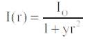
However, the attractiveness β is relative, it should be seen in the eyes of the beholder or judged by the other fireflies. Thus, it will vary with the distance rij between firefly i and firefly j. In addition, light intensity decreases with the distance from its source, and light is also absorbed in the media, so we should allow the attractiveness to vary with the degree of absorption. In the simplest form, the light intensity I(r) varies according to the inverse square law  where Is is the intensity of the source. For a given medium with a fixed light absorption coefficient γ, the light intensity I vary with the distance r. That is I(r), where Io is the original light intensity. In order to avoid the singularity at r = 0 in the expression
 , the combined effect of both the inverse square law and absorption can be approximated using the following Gaussian form.
Light Intensity is,
where I0 is the original light intensity
Intensity I(x) is proportional to the objective function fitness value f(x).
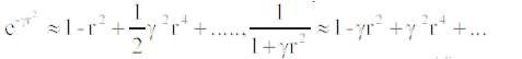
Sometimes, we may need a function which decreases monotonically at a slower rate. In this case, we can use the following approximation.
At a shorter distance, the above two forms are essentially the same. This is because the series expansions about r =0.
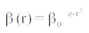
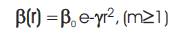
are equivalent to each other up to the order of O(r3). As a firefly's attractiveness is proportional to the light intensity seen by adjacent fireflies, we can now define the attractiveness of a firefly by,
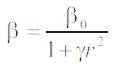
where β is the attractiveness at r = 0. As it is often faster to calculate than an exponential function, the above function, if necessary, can conveniently be replaced by,
In the implementation, the actual form of attractiveness function can be any monotonically decreasing functions such as the following generalized form.
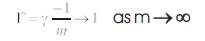
For a fixed , the characteristic length becomes,
Conversely, for a given length scale Г in an optimization problem, the parameter can be used as a typical initial value. That is,
6.2.2 Distance and Movement
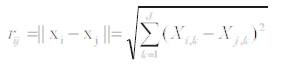
The distance between any two fireflies i and j at Xi and Xj respectively, is the Cartesian distance,
where Xik is the kth component of the spatial coordinate Xi of ith firefly.
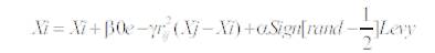
The movement of the firefly i is attracted to another more attractive (brighter) firefly j is determined by,
where the second term is due for the attraction and the third term is randomization via levy flights with α being the randomization parameter.
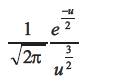
The  where r and ∈ [0,1] essentially provides a random sign or direction while the random step length is drawn from a levy distribution whose mean is infinite and variance is infinite.
The steps of firefly are drawn from a levy distribution random walk with a power law step length distribution with a heavy tail. Furthermore, the randomization term can easily be extended to a normal distribution N (0, 1) or other distributions.
The second term is due to the attraction while the third term is randomization with being the randomization parameter. Rand is a random number generator uniformly distributed in [0, 1].
For most cases in this implementation, we can take β = 1 and α ε [0, 1]. Furthermore, the randomization term can easily be extended to a normal distribution N (0, 1) or other distributions. In addition, if the scales vary significantly in different dimensions such as −0.001 to 0.01.
6.2.3 Formulation of Levy-Flight Firefly Algorithm (Yang, 2010) [ 13]
Begin
Objective function f(x), x = (x1 , x2 , x3 , …,xd )T
Generate initial population of fireflies x (I = 1, 2, 3, … , i n)
Light Intensity Ii at xi is determined by f(xi)
Defined light absorption coefficient γ
While (t < max generation)
For i = 1 : n, for all n fireflies
For j = 1 : n; for all n fireflies
If (Ij> Ii)
Move firefly i towards firefly j in d-dimensions via., levy
flights
end if
Attractiveness varies with distance rij via., exp (- γ rij )
Evaluate new solutions and update light intensity
end j
end i
Rank the fireflies and rank current best
end while
Post processing and visualization
End
6.3 Choice of the Parameters [12]
For most cases, β0=1, α∈[0,1], γ=1, λ=1.5. The 0 parameter γ which characterizes the variation of attractiveness and its value is crucially important in determining the speed of convergence and how FA algorithm behaves. In theory γ∈[0,∞ ] in practice determined by Γ. The characteristic length of the system is to be optimized. Thus, in most cases γ varies from 0.01 to 100.
6.4 Connectivity Analysis
In case of 3-d continuum as in Figure 1, a check for face connectivity between two solid elements is required to ensure that the element will carry the stress. In other words, starting from the seed elements (elements that always carry material such as supports, loads), check for the face connectivity which means two elements having one face in common between them to ensure connectivity between the elements in the continuum. Two elements having an edge or a corner node in common will not be included further in the FE analysis. This is because such elements cannot transfer any moment, and the density, Young's modulus of such elements will be reduced to the order of say 10e-5 , but these elements will participate in the next cycle to generate the newer child population.
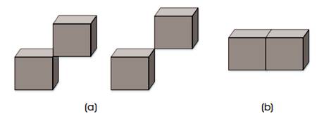
Figure 1. Examples for Solid Elements, not Connected and Connected [3]
7. Discussion of the Study
A program in VC++ is used to perform the finite element analysis. The program consists of two main modules. One is Finite element module and the other is Optimizer module.
7.1 Finite Element Module
Connectivity analysis is performed in case of both plane and solid elements. The connectivity analysis will remove all the elements that have a relative density of 1e-5 , elements connected by corners and also all the isolated elements as well. The distribution of material along with the load and support conditions will be solved further for displacements by using the finite element analysis.
The stresses are calculated for each element in all the points of integration Gauss points, and the centroid as well. The principal stresses are calculated and checked with the maximum permissible stress.
7.2 Optimizer Module
An Optimizer module is a module in which a new set of normalized densities is assigned to each element. In this paper, Firefly algorithm is being used to generate the new set of normalized densities.
7.3 Optimization Process
The optimization is done using Fire Fly Algorithm and two Finite Element Analysis (FEA) approaches. In the first FEA, the stress values are computed for each element at all Gauss points and the centroid of each element. The stress values are checked with the permissible stresses, the principal stresses are computed as the Eigen values of the stress matrix. Error component can be calculated if the stress values exceed the permissible stress. The flowchart for the optimization process is illustrated in Figure 2.
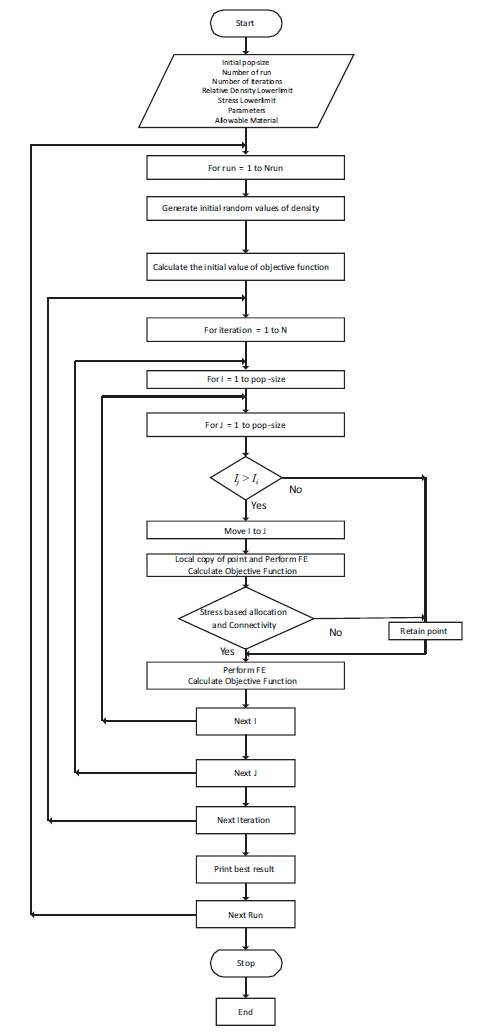
Figure 2. Flowchart for the Optimization Process
This step should identify all the elements that can carry material during the second FEA. If the stresses are below the lower cut off, i.e., the minimum stress, these elements will be assigned the relative density value as 1e-5 . The relative density of seed element is always made equal to 1, for these elements shall carry material at all times during the entire process of optimization. Connectivity check is done after which the newer values of relative density are assigned for each element. In case the connectivity analysis does not contain any output, then the original point is retained. During the second FEA, the elements having relative density higher than the minimum cut off value are assigned the value of 1, and all the other elements are assigned a value of 1e-5 .
In reality, as there is no change in thickness of the element, the relative density of all the elements having the relative density above the minimum is taken as 1, to depict the reality. The second FEA is done to verify the stress of each element at all Gauss points and centroid to be below the permissible stress limits. In order to analyze the response of the structure at a finer level, one way is to discrete the continuum into a finer mesh which mean higher number of elements and finite element analysis could be prohibitively expensive, one other better way is to compute the stresses at different locations within the element.
The objective function is the weight of the structure calculated using the weight density times volume of the structure. This process is iterative and until the minimum weight of the structure is reached satisfying all the constraints. A few problems in the literature are solved and the results are compared. The point load and the support conditions are distributed over four nodes to avoid the stress concentration.
8. Standard Benchmark Problems
A few standard benchmark problems have been solved and the results are compared. The results thus obtained have been verified using MSC Marc® and Mentat® . The parameters used are, β0= 0.10 and 0.15, α= 0.020 and 0 0.025, γ=1, λ=1.5.
8.1 Michelle Structure
The first example corresponds to the topology optimization of the Michell beam with a central point load. Only one half of the structure is analysed due to symmetry. The structure proposed is 1cm thick and the total load applied is P=25 kN distributed into 4 elements around the central point of the domain. The problems are solved with a mesh of 1800 eight node plane stress quadrilateral elements. The refined mesh is obtained by removing the elements with relative density lower than 0.001. The penalization parameter is taken as 2 in the SIMP formulation.
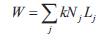
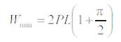
Rozvany in his paper [ 10] gave the formulation for the total weight can be determined using the Primal formulation.
The total weight can also be determined using the Dual formulation.
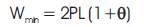
It follows that the optimal total weight becomes,
(for k=ρ /σp = 1, where σp is the permissible stress and ρ is the specific weight)
For a particular case, when angular width tends to zero,
The output in three dimensional view is shown in Figure 3(a). The distribution of material from the point of application of load in the centre to the boundary supports, i.e., the transfer of the load from the point of application to the supports is somewhat unclear. The elements near the edges carry material with relative density varying from 0–1. The elements below the edge carry no material (the relative density is equal to the minimum relative density 0.002) as shown by the thickness of the elements. In reality, the thickness does not vary for each element as shown in the Figure 3(b). The structure will have uniform thickness. The output from the firefly algorithm follows a similar distribution of material. Only one half of the design domain is analysed. The output satisfies the connectivity analysis with two elements having an edge in common. The output is of the form of 1's and 0's, where 1 denotes element carrying full material and 0 denotes elements carrying no material. All the elements below the minimum relative density carry no material and are shown as void.
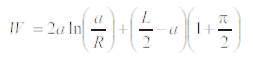
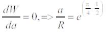
Table1 shows the most important parameters of the problem. The optimal volume of material obtained with the formulation proposed are presented and compared with the optimal ones obtained by Michell. The theoretical minimum volume is calculated using the analytical expression.
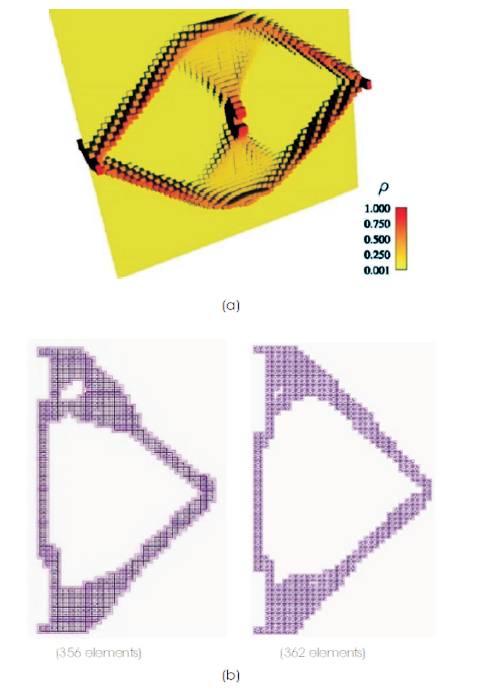
Figure 3. Michelle Structure, (a) Paris et al. (2010), (b) Firefly Algorithm
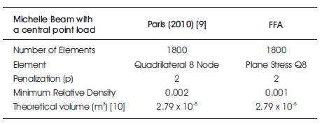
Table 1. Summary of the most important Parameters and Results of the Michelle Beam with a Central Point Load
8.2 A Cantilever Plate
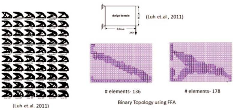
As shown in the Figure 4, a cantilever is subjected to a concentrated load of 3 kN applied at the right hand bottom corner. The nodes on the left hand surface corresponding to the support points were defined to have a zero displacement in the finite element analysis. A design domain is discretised according to 20 x 32 plane stress element FE model. The goal is to minimize the weight satisfying the constraints. The Young's modulus of the material is taken as 200 GPa, Poisson ratio as 0.33, thickness as 0.001 m, and Allowable stress as 200 MPa. The output in the dark black colour on the left side is as given in [ 7] is measured in terms of area varying from 372 (58.125% of V0 ) to 452 (70.6% of V0 ).
Figure 4. A Cantilever Plate Subjected to a Concentrated Load at the Bottom Right Hand Corner
The design domain is a relatively smaller domain, and the applied load is higher. The output obtained using Firefly algorithm is relatively clear and the material is well distributed in the design domain, discussed as follows. The final optimum output has two different distributions. In the first one, linear distribution connecting the supports and the point of application of the concentrated load. The number of elements at the final optimum that carry material is 136 out of a total of 640 elements, 21.25% of the total initial volume of plate. The second distribution as shown on the right side, forms an arch type distribution, connecting the supports with the position of loading. The number of elements carrying material at the final optimum output is 178 out of a total of 640 elements, 27.81% of the total volume of the material.
8.3 L – Shaped Beam
The dimensions of the L-beam are seen in Figure 5, where L = 200 mm and the thickness of the structure is 1 mm. The domain is meshed with 6400 equal sized four node elements and one stress evaluation point is used per element. The super convergent point is used for stress evaluation and for this element type, it is positioned in the centroid of the element. The material is a typical aircraft aluminium with material data; Young's modulus 71000 MPa, density 2.8×10⁻⁹ton/mm3 , Poisson's ratio 0.33, and yield limit 350 MPa. A 1500 N point load is applied as given by Holmberg, (2011).
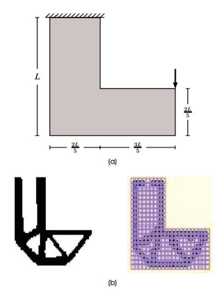
Figure 5 (a) Initial Geometry, (b) After Optimization using FFA
Conclusion
Meta-heuristic algorithms are best suited to perform topology optimisation of continuum structures. In this paper, the existing work done for tuning of algorithms has been extensively reviewed. The Firefly algorithm has been detailed and the parameters that suit have been discussed in greater detail. NP Hard problems which usually require lots of computational effort are reviewed. Few problems are solved using the optimum set of parameters and the results are compared. This study definitely proves a point that meta-heuristics is one of the best ways to perform topology optimisation. Further study can be done by using multi population search engines to explore and exploit the search domain to identify the optimum distribution of material.
Acknowledgement
The authors sincerely thank everyone who helped them complete this paper and review.
References
[1]. Christensen, P.W., and A. Klarbring, (2009). An Introduction to Structural Optimisation. Springer.
[2]. Holmberg, E., B. Torstenfelt, and A. Klarbring, (2013). “Stress constrained topology optimization”. Structural and Multidisciplinary Optimization, Vol. 48, No. 1, pp. 33-47.
[3]. Hsu, M.H., and Y.L. Hsu, (2005). “Generalization of Twoand Three-dimensional structural topology optimization”. Engineering Optimization, Vol. 37, No. 1, pp. 83-102.
[4]. Jakiela, M.J., C. Chapman, J. Duda, A. Adewuya, and K. Saitou, (2000). “Continuum structural topology design with genetic algorithms”. Computer Methods in Applied Mechanics and Engineering, Vol. 186, No. 2, pp. 339-356.
[5]. Li, L., and M.Y. Wang, (2014). “Stress isolation through topology optimization”. Structural and Multidisciplinary Optimization, Vol. 49, No. 5, pp. 761-769.
[6] Lin, C.Y., and F.M. Sheu, (2009). “Adaptive volume constraint algorithm for stress limit-based topology optimization”. CAD Computer Aided Design, Vol. 41, No. 9, pp. 685-694.
[7]. Luh, Guan Chun., Kin, Chun-Yi., and Lin, Yu Shu., (2011). “A binary particle swarm optimization for continuum structural topology optimization”. Applied Soft Computing, Vol.11, No. 2, pp. 2833-2844.
[8]. Pal, S.K., C.S. Rai, and Amrit Pal Singh, (2012). “Comparative Study of Firefly Algorithm and Particle Swarm Optimisation for Noisly Non-Linear optimisation Problems”. International Journal of Intelligent Systems and Applications, Vol. 4, No. 10, p. 50.
[9]. París, J., F. Navarrina, I. Colominas, and M. Casteleiro, (2010). “Improvements in the treatment of stress constraints in structural topology optimization problems”. Journal of Computational and Applied Mechanics, Vol. 234, No. 7, pp. 2231-2238.
[10]. Rozvany, G.I.N., Gollub, W., and Zhou, M., (1997). “Exact Michell layouts for various combinations of line supports – Part II”. Structural and Multidisciplinary, Optimization, Vol. 14, No. 2, pp. 138-149.
[11]. Sui, Y.K., X.R. Peng, J.L. Feng, and H.L. Ye, (2006). “Topology optimization of structure with global stress constraints by Independent Continuum Map method”. International Journal of Computational Methods, Vol. 3, No. 3, pp. 295-319.
[12]. Yang, X.S., (2009). “Firefly algorithms for multimodal optimization”. Lecture Notes in Computer Science (including subseries Lecture Notes in Artificial Intelligence and Lecture Notes in Bioinformatics), pp. 169-178.
[13]. Yang, X.S., (2010). “Firefly algorithm, Lévy flights, and global optimization”. Research and Development in Intelligent Systems XXVI: Incorporating Applications and Innovations in Intelligent Systems XVII, pp. 209-218.
[14]. Yang, X.S. et. al, (2013). “A framework for self-tuning optimisation algorithm”. Journal of Neural Network Computing and Applications, Vol. 23, No. 7-8, pp. 2051- 2057.
[15]. Yang, X.S., (2014). “Swarm intelligence based algorithms: A critical analysis”. Evolutionary Intelligence, Vol. 7, No. 1, pp. 17-28.
[16]. Zang, H., S. Zhang, and K. Hapeshi, (2010). “A review of nature-inspired algorithms”. Journal of Bionic Engineering, Vol. 7, pp. S232-S237.