(1)
In this paper, the authors present an illustratived step by step approach to perform Isogeometric analysis (IGA). The existing literature does not have any solved problems in a stepwise procedure, which can be useful to explain in a classroom. This paper should serve as a benchmark example to refer the stepwise procedure to learn IGA. The focus is on the illustrative stepwise analysis and Isogeometric analysis using NURBS basis functions (Non-Uniform Rational), which can represent the Geometry of the structure more precisely over the finite element method. In this paper, a two dimensional plane plate structure carrying in-plane loading is analysed using Isogeometric analysis. The problem is also solved using Marc Mentat®, a finite element package and the results are compared and presented. The results show that the nodal displacements calculated using Isogeometric analysis are in close agreement with the nodal displacements found using a standard finite element package.
The Isogeometric analysis unifies the fields of CAD (Computer Aided Design) and FEA (Finite Element Analysis). The computational geometry and the computational mechanics have become a sophisticated and complex discipline, but the essence of the finite element method is quite simple and straightforward. The isogeometric analysis capabilities to the existing finite element computer programs can include on a wide variety of applications. The unique feature of Isogeometric analysis which is not available in the traditional finite element analysis is the exact representation of the geometry in the engineering design. The features of CAD and FEA is much closer and Isogeometric analysis will unify these fields. Hughes et al. (2005) in his paper used Rational B-Spline (NURBS) basis functions and discussed their unique properties on a wide variety of applications and how the research on these powerful functions might benefit across several fields. Particular attention is given to the Galerkin finite element method within the framework of Isogeometric analysis.
In this paper, the focus is to present a step wise illustrative approach to perform Isogeometric analysis of a plate structure. The NURBS basis functions were developed by Espath et al. (2011). The basis functions for geometry and displacement are considered to be the same. The Strain Displacement matrix and the Stiffness matrix were developed for each element. The element stiffness matrix is then assembled to form a global stiffness matrix. The global force vector is then formed. The boundary conditions were applied and the nodal displacements were determined. The structure is also analysed using first order four node quadrilateral elements using Marc Mentat®, which is a standard finite element package. The nodal displacements calculated using NURBS based IGA are in good agreement with the nodal displacements calculated using the standard finite element analysis.
The era of parallel computing is on the horizon. The largest mesh simulations have stalled and the adaptive meshes have been increasingly in use. To capatilize on the O(100,000) core parallel systems, CAD, geometry, meshing, analysis, adaptivity, and visualization have to run in a tightly integrated way in parallel in a scalable fashion. To breakdown the barriers between engineering design and analysis and to reconstitute the entire process, the focus on a precise geometric model is the only way. The change from the classical finite element program to the analysis procedure based on CAD representation is referred to as Isogeometric analysis (Hartmann et al., 2011).
Hartmann et al. (2011) studied NURBS in depth and it has been shown that NURBS are well suited for computational analysis in comparison with standard Lagrange polynomials. Hassani et al. (2012) performed Isogeometric analysis to perform structural optimization instead of finite elements. A control point based Solid Isotropic Material with Penalisation (SIMP) is employed approximated by using NURBS. Optimality criteria is derived and developed. Nagy et al. (2010)proposed a novel variational based formulation of stress constraint in their paper. The weak form is used to represent geometry, response variables, design variables, and Lagrange multipliers as well. Volume minimization of elastic arches subjected to stress constraints is considered. Shah and Katukam (2010) in their paper, discussed the basic formulation of 2D plate problems and 3D problems to apply the Isogeometric analysis to perform static analysis of few structures. Lee et al. (2010) developed code to perform structural analysis using Isogeometric concept. The results obtained using Isogeometric analysis have shown a good agreement with the results obtained using NASTRAN®.
The NURBS basis functions and the parent to parametric mapping were discussed (Chandrasekhar et al., 2018). The strain displacement matrix is presented and then the stiffness matrix is formed. An example of a two dimensional plate continuum has been analysed using Isogeometric analysis. The NURBS basis functions are used and discussed. The stiffness matrix is derived in a step wise manner. The solution for the displacement vector at each node is compared with the results from the standard finite element analysis. The results show that the nodal displacement are in good agreement with the results obtained from IGA and the nodal displacements using standard FEA.
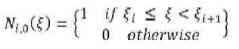
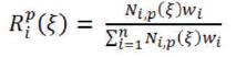
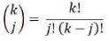
The basis functions are given by,
For p = 1, 2, 3,….
They are defined by,
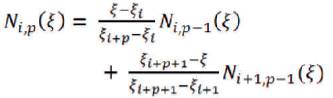
This is referred to as the Cox-de Boor recursion formula (Gondegaon and Voruganti, 2016).
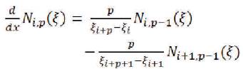
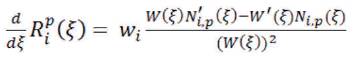
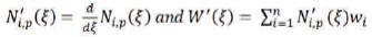
The derivatives of the basis functions are given by,
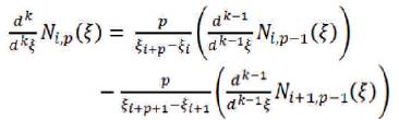
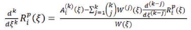
The generalized higher order derivatives of the basis functions (Hughes et al., 2005) is given by,
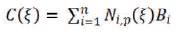
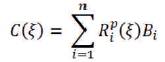
The B-spline curve is given by,
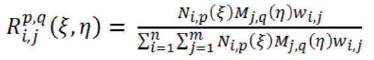
4.4.1 B-spline Surfaces
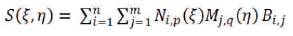
B-spline surfaces is given by,
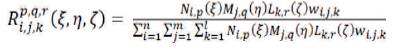
4.4.2 B-Spline Solids
B-spline solids is given by,

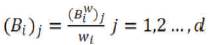
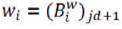
With a given projective B-spline curve and its associated projective control points in hand, the control points for the NURBS curve are obtained by using the following relations (Chandrasekhar et al., 2018).
NURBS basis is given by,
where,
4.5.1 For NURBS Curve
The NURBS curve is given by,
This is identical to the B-Splines.
4.5.2 For NURBS Surfaces
The NURBS surfaces is given by,
4.5.3 For NURBS Solids
The NURBS solids is given by,
4.5.4 Derivatives of NURBS
Apply the quotient rule, the derivatives of NURBS is given by,
where
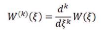
4.5.5 For Higher Order Derivatives of NURBS Basis Functions
The higher order derivatives of NURBS basis functions (Hughes et al., 2005) is given by,
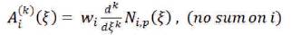
We do not sum on the repeated index, and let
Higher order derivatives can be expressed in terms of the lower order derivatives as,
where,
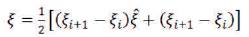
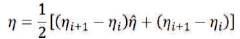
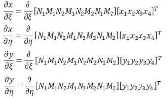
The parametric to parent mapping is given by,
The Jacobian is given by,
4.6.1 Parametric Space to Physical Space
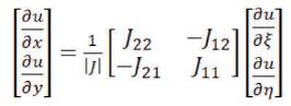
The parametric space to physical space (Gondegaon and Voruganti, 2016) is given by,
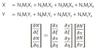
where,
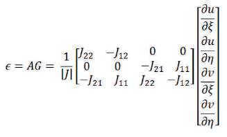
The strain displacement matrix (Chandrasekhar et al., 2018) is given by,
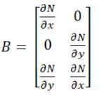
The strain vector is given by
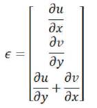
where,
The strain is given by,
4.7.2 Plane Stress
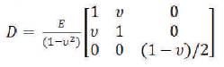
The elasticity matrix for the material in plane stress condition is given by,
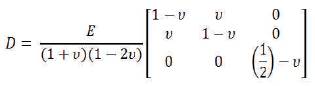
4.7.3 Plane Strain
The elasticity matrix for the material in plane strain condition is given by,
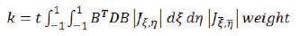
4.7.4 Stiffness Matrix
The stiffness matrix (Nguyen et al., 2015) is given by,
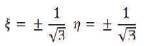
4.7.5 Gauss Quadrature
The Gauss quadrature points are given by,
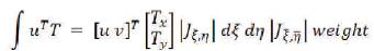
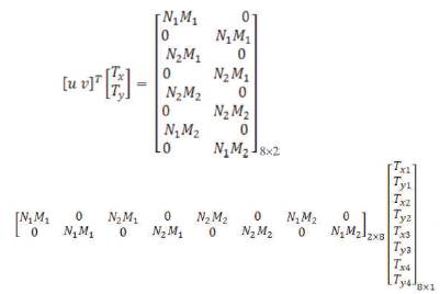
The traction is given by,
The algorithm to perform the Isogeometric analysis of a two dimensional plate structure carrying in-plane loading ( Chandarasekhar et al., 2018;Shah and Katukam, 2010) is given below.
 using elRangeU and elRangeV.
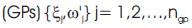 where ngp is the number of gauss points.
(i) Compute parametric coordinate  corresponding to
  .
.
(ii) Compute  corresponding to the equations.
(iii) Compute the derivatives of the shape functions  at point
  .
.
(iv) Compute  using control points (sctr(:,e))
(v) Find  and determinant .
(vi) Compute the shape function derivatives 
 .
.
(vii) Use Rx to build the strain displacement matrix B.
(viii) ke = ke + BTDB  .
.
Although the literature available on Isogeometric analysis is not very exhaustive (Chandrasekhar et al., 2018), the analysis is done in a step wise manner. The existing literature by Chandrasekhar et al. (2018) is reviewed first, and the plate problem is chosen to present the Isogeometric analysis of a plate structure in a step-wise illustrative approach. The basis functions were developed. The strain-displacement matrix and the stiffness matrix, force vector are assembled. The nodal displacements were calculated. The flowchart of Figure 1 shows the approach followed to complete this study, which has been obtained from the previous study conducted by Chandrasekhar et al. (2018).
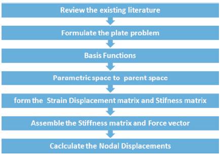
Figure 1. Approach to Conduct this Study (Chandarasekhar et al., 2018)
A two dimensional plate structure as shown in the Figure 2(a) and 2(b) is 20 x 20 mm. The domain is shown in Figure 2(a) and the control net is as shown in Figure 2(b). The domain is discretized into four numbers first order four node quadrilateral elements in plane stress condition. The number of nodes is equal to 9. The right side nodes numbered 3, 6 and 9 are fixed. The Y-displacements at node 1 and node 7 is equal to zero. The Young's modulus of the material is equal to 2e5 MPa and the Poisson's ratio is taken as 0.30. The thickness of the plate is taken as equal to one unit. A horizontal load of 1257 N is applied at node 1 and 7. A horizontal force of 2514 N is applied at node 4 as shown in Figure 2(a). Table 1 shows the control points and knots. Three control points along each axis. The degree of basis function is equal to 1 along each axis.
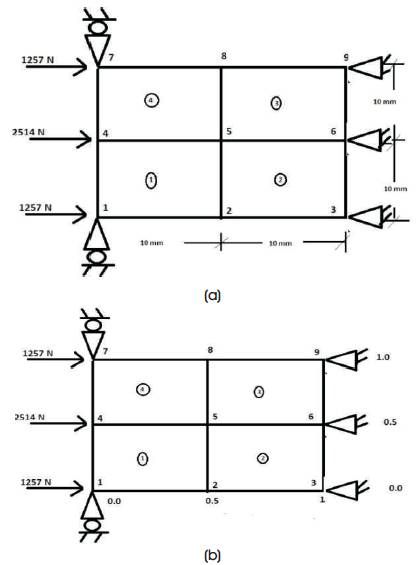
Figure 2. (a) A Two Dimensional Plate Structure, (b) Control Net and Knot Vector
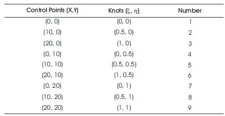
Table 1. Control Points and the Knots
The  vector is
 ={0,0,0,0.5,1,1,1} and Eta(
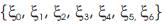 ) vector is
  ={0,0,0,0.5,1,1,1} . The degree of basis function along direction (p) and
  direction (q) is equal to 1. p=q=1.
NURBS basis functions are given by,
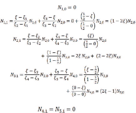
The NURBS basis functions are given in Table 2.
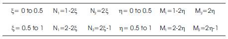
Table 2. NURBS Basis Functions
The element wise nodes and integration points are given in Table 3.
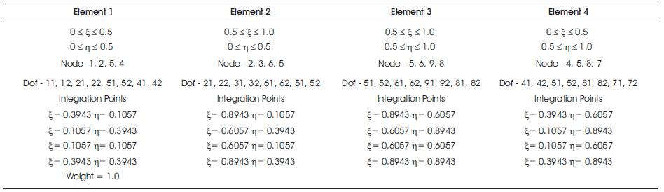
Table 3. Element Wise Knots, Degree of Freedom (DOF) and the Integration Points
The step-wise procedure to form the stiffness matrix is discussed in this section.
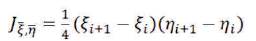
6.2.1 Parametric Space to Parent Space
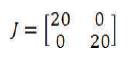
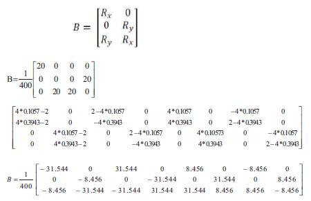
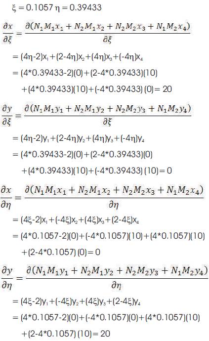
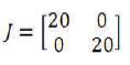
The Jacobian for mapping parametric space to parent space is given by,
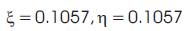
The Gauss points of integration in parametric space are given in Table 4.
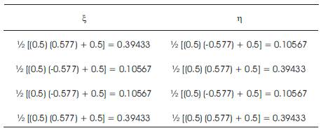
Table 4. Gauss Integration Points in Parametric Space
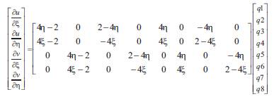
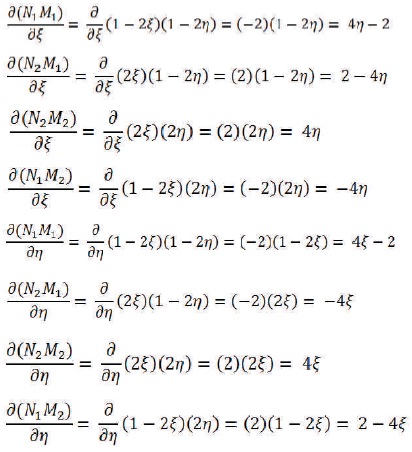
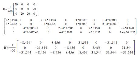
The first derivatives in parametric space are given by
6.2.2 For Gauss Point 1
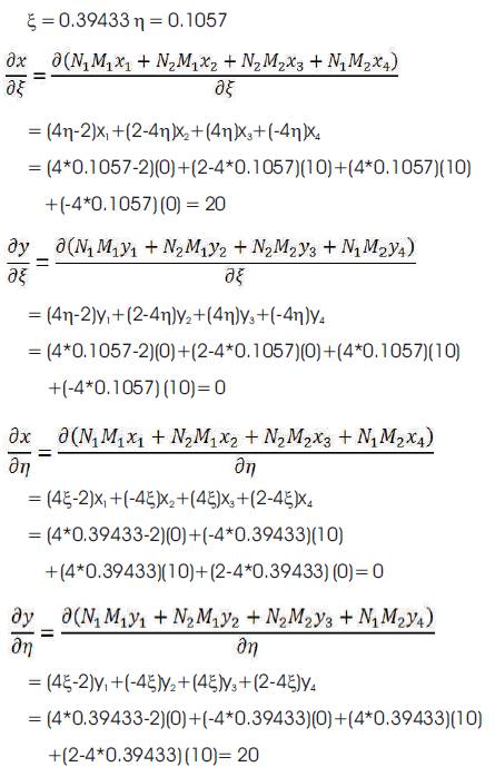
The Jacobian is given by,
The numerical integration is performed at four Gauss points for each element in the following sub-sections.
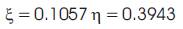
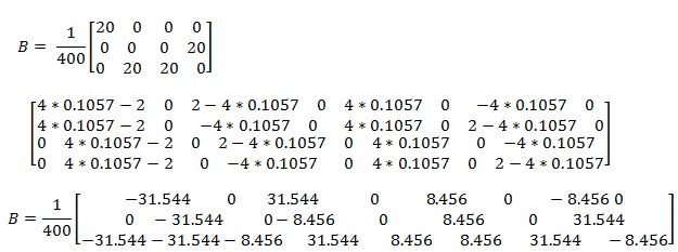
6.2.2.1Numerical Integration
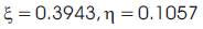
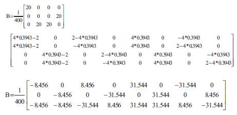
The strain displacement matrix is given by,
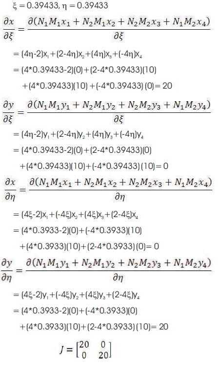
6.2.3 For Gauss Point in the Parametric Coordinates
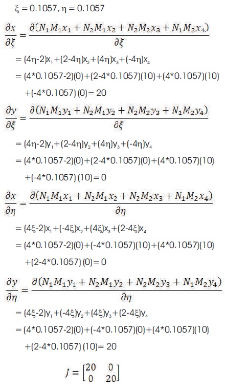
The Jacobian is given by,
6.2.3.1Numerical Integration
The strain displacement matrix is given by,
6.2.4 For Gauss Point in the Parametric Coordinate System
6.2.4.1 Numerical Integration
The strain displacement matrix is given by,
6.2.5 For Gauss Point
6.2.5.1Numerical Integration
The strain displacement matrix is given by,
6.3 Stiffness Matrix
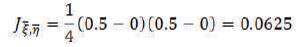
Multiplier for element stiffness matrix 
The stiffness matrix is calculated using equation (28) as follows.
6.3.1 Element 1
The stiffness matrix is calculated at each integration point is tabulated in Table 5.
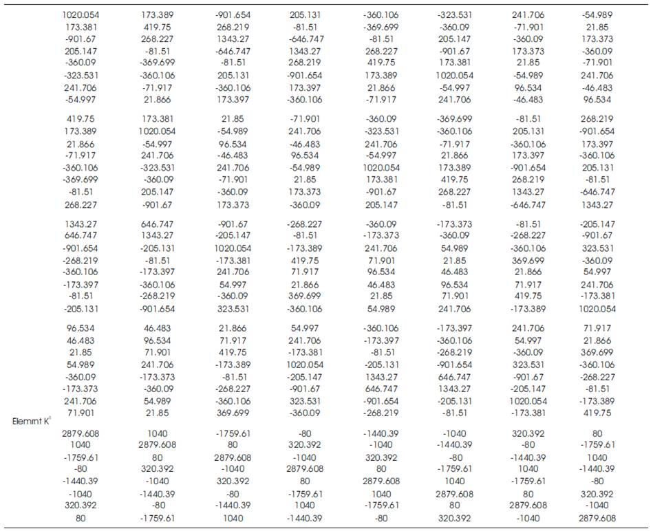
Table 5. Stiffness Matrix at Each Integration Point
6.3.2 For Element 2
The basis functions for element 2 are given in Table 6.

Table 6. NURBS Basis Functions for Element 2
The stiffness matrix is calculated at each integration point and given in Table 7.
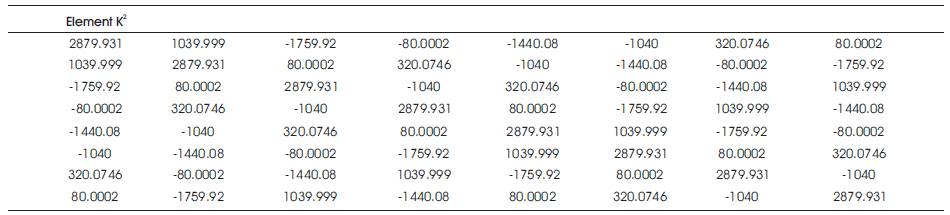
Table 7. Stiffness Matrix for Element 2
6.3.3 For Element 3
The basis functions for element 3 are given in Table 8. The stiffness matrix is calculated at each integration point and given in Table 9.

Table 8. NURBS Basis Functions for Element 3
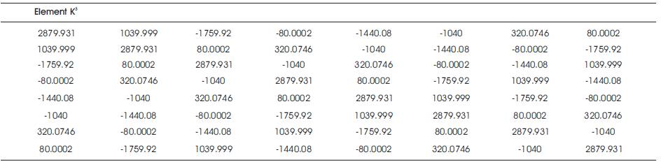
Table 9. Stiffness Matrix for Element 3
6.3.4 For Element 4
The basis functions are given as in Table 10.

Table 10. NURBS Basis Functions for Element 4
The stiffness matrix is calculated at each integration point and given in Table 11.
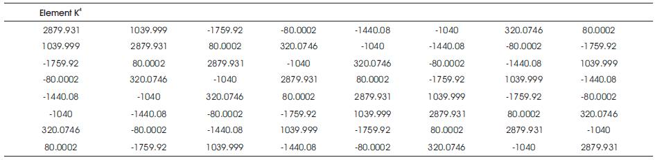
Table 11. Stiffness Matrix for Element 4
6.3.5 Boundary Conditions
The boundary conditions are applied,
The rows and columns are eliminated from the stiffness matrix and the rows having zero displacements from the force vector are eliminated. The reduced stiffness matrix and the force vector are given in the next section.
The reduced stiffness matrix is as shown in the Table 12
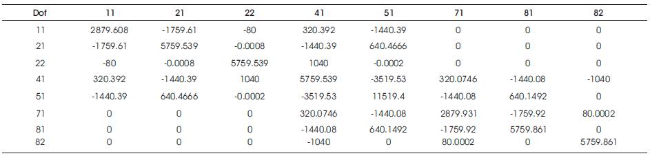
Table 12. Reduced Stiffness Matrix
The reduced force vector is shown in Table 13.

Table 13. Reduced Force Vector
The relation KGUG = FG is solved to determine the nodal G displacements (UG ).
The nodal displacements are given. The structure is analysed in Marc® using first order four noded quadrilateral elements and the nodal displacements are given in Table 14.
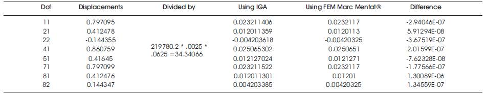
Table 14. Nodal Displacements using IGA and FEA
6.6.1 Analysis using Marc®
The results show that the nodal displacements calculated using Isogeometric Analysis are in close agreement with the results obtained using standard Finite Element Method using Marc Mentat® as shown in Figure 3 and Figure 4.
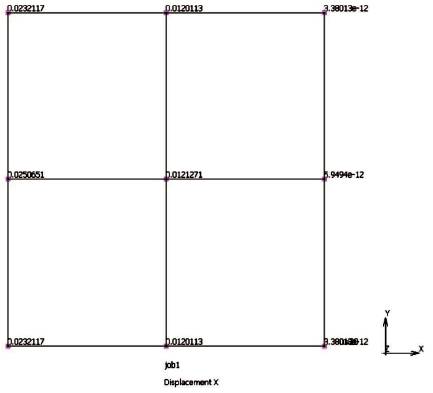
Figure 3. Nodal X-Displacements for the Two-Dimensional Plate Structure using Finite Element Analysis Package Marc Mentat®
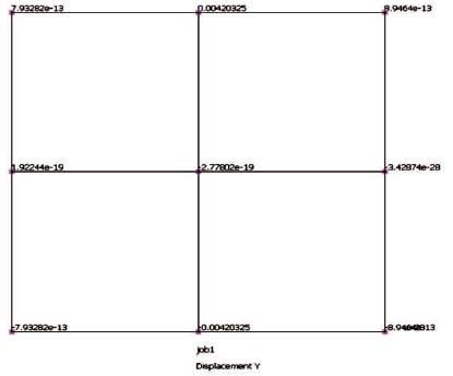
Figure 4. Showing the Nodal Y-Displacements for the Two-Dimensional Plate Structure using Finite Element Analysis Package Marc Mentat®
The NURBS basis functions were discussed in the theoretical background. The literature review is not included to limit the number of pages. However, the analysis section is elaborately discussed. The step by step illustrative procedure is clearly explained here. The derivation of the basis function, the mapping from the parent space to parametric space is clearly explained. The strain displacement matrix is derived for each element and the stiffness matrix is formulated for each element. The global stiffness matrix is assembled and the system of simultaneous linear equations are solved to find the nodal displacements. The nodal displacements obtained using Isogeometric analysis are in close approximation to the nodal displacements obtained by analyzing the plate structure using MARC Mentat®, a commercial standalone package. The authors hope, this paper can be useful as a classroom example.
Isogeometric analysis can be further extended to analyse problems in shell structures and fracture mechanics. Isogeometric analysis can be useful to analyse complex geometry such as medical imaging as well.