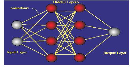
Figure 1. Structure of ANN
Increased interconnectlon of the power system along with deregulated structure to satisfy growing demand has brought new challenges for power system state estimation. The estimation of power system state [1, 3] in such interconnected system has become complex due to complexity in modelling and uncertainties. This makes ANN a ideal candidate for state estimation, since it can accurately map the relationship between the measured variable and other state variables of the power system with reduced computational resources as compared to weighted least square approach[2]. Using only load bus parameters for various operating conditions with an ANN other states of the power system can be accurately estimated. This paper discusses an approach to estimate the state of power system using ANN in MATLAB.
The definition of a neural network, more precisely referred to as an 'Artificial' Neural Network (ANN), is provided by the inventor of one of the first neurocomputers, Dr. Robert Hecht-Nielsen. He defines a neural network as:
"A computing system made up of a number of simple, highly interconnected processing elements, which process information by their dynamic state response to external inputs".
Neural networks are basically organized in layers and these layers are made up of a number of interconnected 'nodes' which contain an 'activation function'. System data are presented to the network via the 'input layer', which communicates to one or more 'hidden layers' where the actual processing is done via a system of weighted 'connections'. The hidden layers is link to an 'output layer' where the output results are as shown in the Figure 1 .
Figure 1. Structure of ANN
ANNs contain some form of 'learning rule' which modifies the weights of the connections according to the input patterns that it is presented [4]. In a sense, ANNs learn by examples as do their biological counterparts; a child learns to recognize dogs from examples of dogs. More simply, when a neural network is initially presented with a pattern it makes a random 'guess' as to what it might be. It then sees how far its answer was from the actual one and makes an appropriate adjustment of its connection weights.
Learning in a neural network is called training. Like training in athletics, training in a neural network requires a coach, Someone that describes to the neural network what it should have produced as a response. From the difference between the desired response and the actual response, the error is determined and a portion of it is propagated backward through the network[5]. At each neuron in the network the error is used to adjust the weights and threshold values of the neuron, so that the next time, the error in the network response will be less for the same inputs.
This corrective procedure is called back propagation (hence the name of the neural network) and is applied continuously and repetitively for each set of inputs and corresponding set of outputs produced in response to the inputs is shown in Figure 2. This procedure continues so long as the individual or total errors in the responses exceed a specified level or until there are no measurable errors, At this point, the neural network has learned the training material and you can stop the training process and use the neural network to produce responses to new input data.
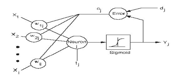
Figure 2. Neural network training
There are various training algorithms in MATLAB using which ANN can be trained to achieve the best fit.
The Levenberg-Marquardt algorithm is designed to approach second-order training speed without computing the Hessian matrix. When the performance function has the form of a sum of squares then the Hessian matrix can be approximated as H = JTJ.
The gradient can be computed as g = JTe.
where J is the Jacobian matrix that contains first derivatives of the network errors with respect to the weights and biases, and e is a vector of network errors.
The Levenberg-Marquardt algorithm uses this approximation to the Hessian matrix in the following Newton-like update:
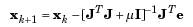
When the scalar µ is zero, this is just Newton's method, using the approximate Hessian matrix. When µ is large, this becomes gradient descent with a small step size. Newton's method is faster and more accurate near an error minimum, so the aim is to shift toward Newton's method as quickly as possible. Thus, µ is decreased after each successful step (reduction in performance function) and is increased only when a tentative step would increase the performance function. In this way, the performance function is always reduced at each iteration of the algorithm.
'trainlm' is a network training function in MATLAB corresponding to Levenberg-Marquardt training algorithm,
Back propagation is used to calculate derivatives of performance perf with respect to the weight and bias variables X. Each variable is adjusted according to the following:
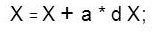
where dX is the search direction. The parameter a is selected to minimize the performance along the search direction. The line search function search Fcn is used to locate the minimum point. The first search direction is the negative of the gradient of performance, In succeeding iterations the search direction is computed from the new gradient and the previous search direction according to the formula,
where gX is the gradient. The parameter Z can be computed in several different ways.
'trainscg' is a network training function in MATLAB corresponding to Scaled conjugate gradient back propagation.
Bayesian regularization minimizes a linear combination of squared errors and weights. It also modifies the linear combination so that at the end of training the resulting network has good generalization qualities.
This Bayesian regularization takes place within the Levenberg-Marquardt algorithm, Back propagation is used to calculate the Jacobian jX of performance perf with respect to the weight and bias variables X. Each variable is adjusted according to Levenberg-Marquardt,
where E is all errors and I is the identity matrix.
'trainbr is a network training function in MATLAB corresponding to Bayesian regulation back propagation.
The default network for function fitting (or regression) problems, fitnet, Is a feed forward network with the default tan-sigmoid transfer function in the hidden layer and linear transfer function in the output layer. The authors assigned ten neurons (somewhat arbitrary) to the one hidden layer in the previous section. The network has one output neuron, because there is only one target value associated with each input vector.
net = network{ , . .
1, . . . % numlnpUts, number of inputs,
2, . . . % numLayers, number of layers
[ 1 ; 0], . . . % biasConnect, numLayers-by-1 Boolean vector,
[ 1 ; 0], . . . % inputConnect, numLayers-by-numlnputs
Boolean matrix,
[0 0; 1 0], ... % layerConnect, numLayers-by-numLayers
Booleanmatrix
[0 1 ] , . . % outputConnect, 1-by-numLayers Boolean
vector);
%number of hidden layer neurons
net.layers { 1 } .size = 10;
% hidden layer transfer function
net.layers{ 1 } .transferFcn = 'logsig';
net = configure(net,inputs,targets);
% initial network response without training
initial_output = net(inputs)
The network uses the default Levenberg-Marquardt algorithm (trainlm) for training. For problems in which Levenberg-Marquardt does not produce as accurate results as desired, or for large data problems, consider setting the network training function to Bayesian Regularization (trainbr) or Scaled Conjugate Gradient (trainscg), respectively, with either.
net.trainFcn = 'trainlm';
net.performFcn = 'mse';
[net,tr]= train(net,inputs,targets);
%network response after training
final_output = net(inputs)
%View network structure
view(net);
After the network has been trained, you can use it to compute the network outputs. The following code calculates the network outputs, errors and overall performance.
outputs = net(inputs);
errors = gsubtract(outputs, targets);
performance = perform(net,targets,outputs)
figure, plotperform(tr)
figure, plottrainstate(tr)
figure, plotregression(targets,outputs)
figure, ploterrhist(errors);gensim(net)
Table 1 to 4 give the generator, line and load data for IEEE 6 bus system

Table 1. Load Data
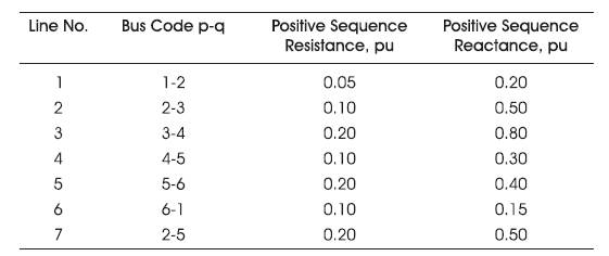
Table 2. Line Data
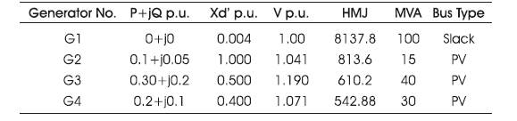
Table 3. Generator Data
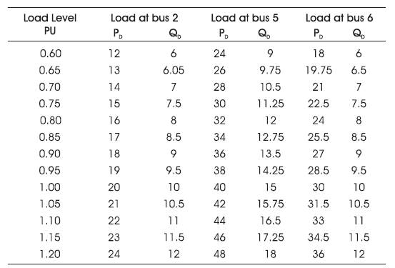
Table 4. Load Level & Loads at Each Bus
The IEEE 6 bus system is simulated in PSAT as shown in Figure 3. The input and target sets are prepared by considering 10 load conditions, corresponding real and reactive powers are considered as inputs and bus voltage and magnitudes are considered as outputs and data sets are loaded first to excel sheet and then they are imported to MATLAB for training an ANN . The sizes of both matrices are 20X 12 as there are 6 buses.

Figure 3. Simulated Diagram in PSAT
65%, 70%, 75%, 80%, 85%, 90%, 95%, 100%, 105% . (Ten Rows)
close all, clear all, clc, format compact
inputs 1 = xlsread('C:\Users\admin\Desktop\phase
2\simulations\example2\inputs.xlsx','Sheet 1 ');; % input
vector
targets 1 = xlsread('C:\Users\admin\Desktop\phase
2\simulations\example2\targets.xlsx','Sheet1');
inputs = inputs1';
targets = targets1';
%corresponding target output vector
%create network
net = network( . . .
1, . , . % numinputs, number of inputs,
2, . , . % numLayers, number of layers
[1; 0], . , . % biosConnect, numLayers-by-1 Boolean vector,
[1; 0], .. % inputConnect, numLayers-by-numlnputs Boolean matrix,
[0 0; 1 0], % layerConnect, numLayers-by-numLayers Boolean
matrix
[0 1] .., % outputConnect, 1-by-numLayers Boolean
vector
); % number of hidden layer neurons
net,Iayers {1 } .size = 10;
% hidden layer transfer function
net. layers { 1 } . transfer Fcn = 'tansig'; net =
configure(net,inputs,targets);
%initial network response without training
initial_Output = net(inputs) % network trainlng
net.trainFcn = 'trainlm'; net.performFcn = 'mse';
[net,tr] = train(net,inputs,targets);
% network response after training
final_output = net(inputs)
view(net); % View network structure
%Test the Network
outputs = net(inputs);
errors = gsubtract(outputs,targets);
performance = perform(net,targets,outputs)
figure, plotperform(tr); figure, plottrainstate(fr)
% figure, plotfit(net, targets 1 ,outputs)
figure, plotregression(targets,outputs);
figure, ploterrhist(errors); gensim(net);
Results: The regression and error histogram for above trained network are shown in Figure 4 and 5 .
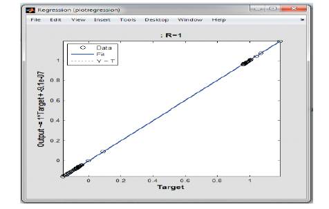
Figure 4. Regression Plot
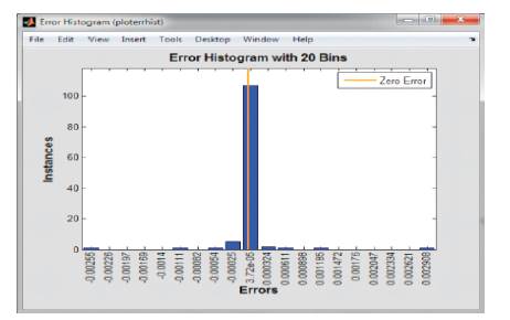
Figure 5. Error Histogram
The above system is further trained by changing the number of neurons in the hidden layer and the results are given in Table 5. Figure 4 shows the Regression Plot. Figure 5 shows the Error Histogram. Figure 6 represents the Simulink diagram and Figure 7 shows the Trained Neural Network.
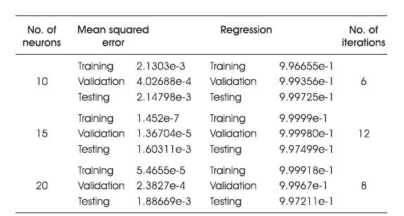
Table 5. Effect of Number of Neurons in Hidden Layer
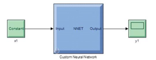
Figure 6. Simulink Diagram
Levenberg-Marquardt back propagation
The above system is further trained by considering other training algorithms and results are given in Table 6 .
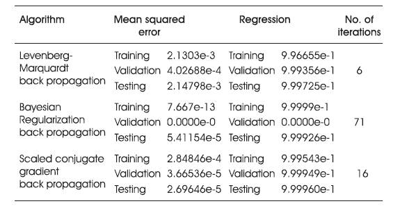
Table 6. Effect of Various Learning Algorifhms
Instead of considering only 10 load levels as in the previous case, now 20 load levels are considered and network is trained again and the corresponding results are as shown in Figure 8, the regression plot and error histograms are provided in Figure 9 and 10:
63%,65%,67%,70%,73%,75%,80%,83%,85%,87%,90% , 93%,95%,97%, 100%, 103%, 105%, 113%. 117%.
It can be observed that with increased data size the performance of the network still improved both in terms of regression and mean squared error.
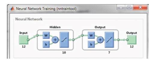
Figure 7. Trained Neural Network
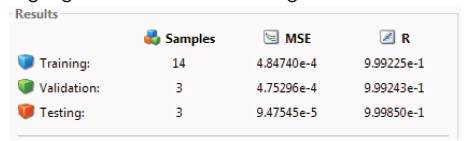
Figure 8. Results of 20 Load levels
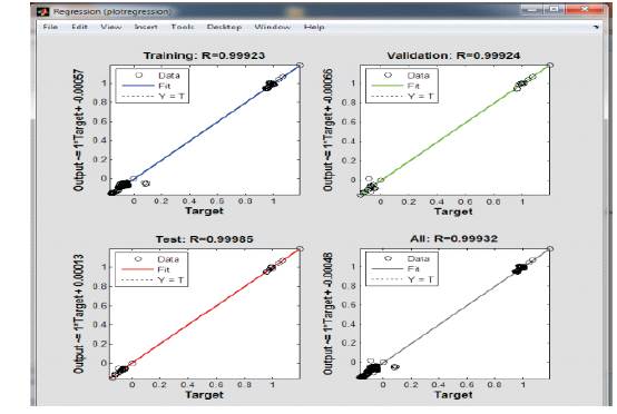
Figure 9. Regression Plot
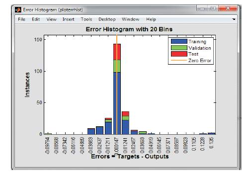
Figure 10. Error Histogram
Once the Trained Network is Satisfactory then the output for other situations can be obtained by making use of generated simulink diagram given in Figure 11 .
After providing the inputs (real and reactive powers for required loading conditions) the output plot is generated as shown in Figure 12 and corresponding data can be imported to workspace also.
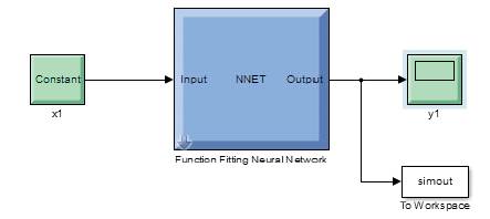
Figure 11.Generated Simulink Diagram
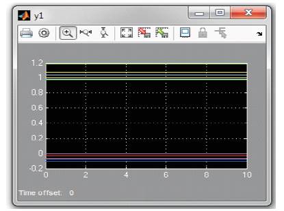
Figure 12. Simulink Output for 60% Load Level
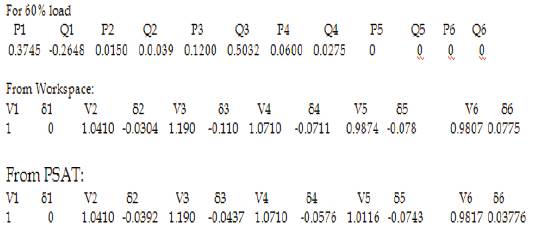
It can be observed from the above results that the network has been trained to maximum accuracy and is able to estimate the state of the system for other load conditions also.
The IEEE 14 bus system is simulated using PSAT as shown in Figure 13 .

Figure 13. IEEE 14 Bus Simulated Diagram in PSAT
The Input and target sets are prepared by considering 20 load conditions in a similar way as explained for 6 bus system. The sizes of both matrices are 20X28 as there are 14 buses. The MATLA8 code has been written to train the network by using Levenberg-Marquardt backpropagation algorithm.
The corresponding neural network which is generated is shown in Figure 14.
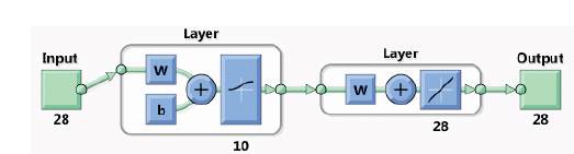
Figure 14.Neutral Network corresponding to 14 Bus System
Results: The regression and error histogram plots for above trained network are given in Figures 15 and 1 6 .
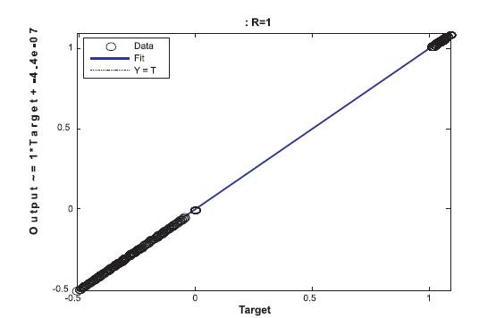
Figure 15. Regression Plot
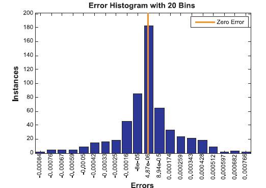
Figure 16. Error Histogram
The value of regression being 1 it shows that the network training has been trained to provide best estimates. Also by observing error histogram it is clear that errors are almost near zero error line and they are considerably less as we move away from zero error line.
The trained network is considered for estimating the state of the system for 100% load and results are tabulated in Table 7 along with results from Mipower software and PSAT. The corresponding plots showing these results are given in Figures 17 and 18.
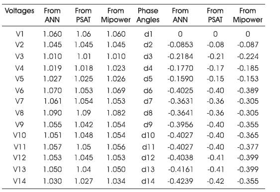
Table 7. Tables of system for 100% Load
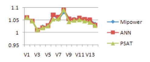
Figure 17. Bus voltages for above three references
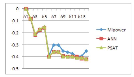
Figure 18. Bus angles for above three references
Power system state estimation which is an important aspect of power system control and operation has been explained in this paper using ANN toolbox of MATLAB. An IEEE 6 bus system is considered and has been modelled using PSAT and results are used to train the ANN. Various learning algorithms with various number of neurons in the hidden Layer are considered for training and the results are tabulated. Based upon the mean squared error and regression, the algorithm and number of neurons in the hidden layer can be chosen for required application.