Mobile ad hoc networks[1-3] collective agreement of the mobile nodes that can communicate with each other without the aid of any centralized point. Ad-hoc networks make a practical and effective use of multi-hop radio transmission and radio communication channel. It [4] is very important for a mobile host to seek help from other hosts in forwarding a packet to its destination, due to limited transmission range of each mobile node. With improved technology, this network could be managed by end users rather than authority and can only be used for extremely sensitive applications. In ad-hoc networks, node mobility is an important issue because of the adhoc features such as dynamic network topology, shared medium, bandwidth limited, the multi-hop and security, etc. So, not a prerequisite for effective management plan for mobility, i.e. mobility without the ad-hoc networks. Seamless mobility provides an easy and effective communication between the nodes in the network. A mobile ad-hoc network (MANET) is an autonomous system of mobile nodes connected by wireless links. In a MANET is assumed that the nodes are free to move and are able to communicate with each other, often through multi-hop links, without the aid of a fixed network infrastructure.

The network topology is dynamic. The movements of a node or the communication range of the nodes of other changes not only its neighborly relations with the other nodes, but also change all the routes on the basis of these relations. Traffic signaling overhead for the establishment and maintenance of routes in a MANET is proportional to the rate of change of this link. Therefore the performance of a MANET is closely related to the efficiency of routing protocol in adapting to changes in network topology and link state[5,6]. To evaluate the performance of a protocol Routing for a MANET, it is essential to use a mobility model suitable to simulate the motion of the nodes in a network[7]. The authors present some mobility models have been proposed or used in evaluating the performance of adhoc network protocols. The models presented are the benchmark model of random mobility[5], the Gauss- Markov random [8,9] and the reference point group mobility model [10].

Mobility models in ad-hoc networks represent[10] the movement pattern of mobile users and how the change of location, speed, direction and acceleration in time. In these networks, mobile nodes communicate directly with each other. Communications between two nodes do not produce effective results if both nodes are not in the same transmission range. This problem can be solved by using intermediate routing nodes. Therefore, routing is very important for mobile ad-hoc networks where mobility models should be evaluated with respect to the end to end delay and efficient data transmission. Mobility models are intended to focus on individual movement patterns due to the point to point communication over cellular networks[9,11,12], while ad-hoc networks are designed for group communication. These models [13] are suggested to keep moving, and efficient transmission between nodes in real-life applications. Besides, these models are mainly focused on the behavior of individual movement between the era of mobility with minimum time simulation in which a mobile node moves with constant speed and direction. These models represent the characteristics of mobile nodes in an ad-hoc as speed, direction, distance and motion of the node. Mobility models[7] can be classified based on the following criteria based on the size, scale, mobility, fate, geological constraints, destiny and guided by the change of parameters (discussed in the next section). In general, there are two types of mobility models (i) Tracebased mobility models and (ii) synthetic mobility models. Trace models provide mobility patterns based on the deterministic approach while synthesis models shows the movements of mobile nodes in a realistic way.

1.1 Random Waypoint Model

Johnson and Maltz model to describe the random reference point (RRP) in [5]. In this model, a node randomly selects a destination uniformly distributed in a predefined area, and moves to that destination at a speed of chance, which is also distributed uniformly between predefined minimum and maximum speed to reach its destination. After a pause for a period of time, the node selects a new random destination and speed. A typical trajectory of a node moves in the model of random reference point shown in Figure 1.

Figure 1. Random Reference Point (RRP)

1.2 Random Gauss-Markov Model

The Random Gauss-Markov (RGM) Model was described by Sanchez[14] and was developed by Liang and Haas[15]. In this model, each node is assigned a speed s and direction q and these variables are updated at each time step Δt as follows,

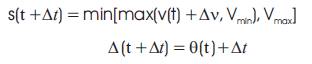
Here V_min and V_max are the minimum and maximum speeds  of the node, and Δν and Δθ are random variables uniformly distributed over the intervals [-Δν_max, Δν_max] and  [-Δθ_max, Δθ_max], respectively. When a node reaches a boundary, the node is reflected from that boundary by the selection of a new random direction. The update of S and q can be implemented in various ways. A typical trajectory of a node moving in a random Gauss-Markov Model is shown in Figure 2.

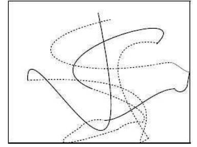
Figure 2. Random Gauss-Markov Model (RGM)

1.3 Reference Point Group Mobility

The Reference Point Group Mobility (RPGM) model was described by Hong et al in[11]. In the RPGM model, node group has center of logic, which defines characteristics of the group movement such as location, speed and direction. Thus, the trajectory of a group is determined by the trajectory of its central logic.

In addition to the center of logic, the model RPGM defines a reference point and a random motion vector for each node in the group. A benchmark is a point on which a node moves randomly with respect to the center of logic. The random motion vector representing random deviation of a node from the point of reference.

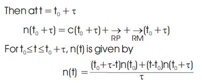
The random motion vector is updated periodically and its magnitude and direction are uniformly distributed over the intervals [0, RM_max ] and [0, 2π] respectively. Let n(t₀ ) be the  location vector of a node of the RPGM model at t = t₀ , then

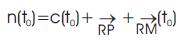
Where c(t₀ ) denotes the location vector of the logical  center of the group at time is a vector from the logical center to the reference point, and    is the  random motion vector.

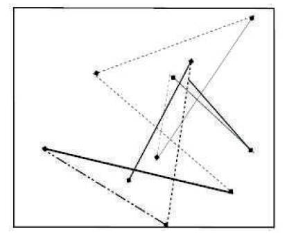
A typical trajectory of a node moving in the RPGM model is shown in Figure 3.

Figure 4 Depicts the movement of the RPGM model for a group with three nodes.

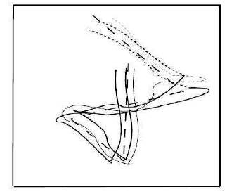
Figure 3. RPGM model (3 nodes)

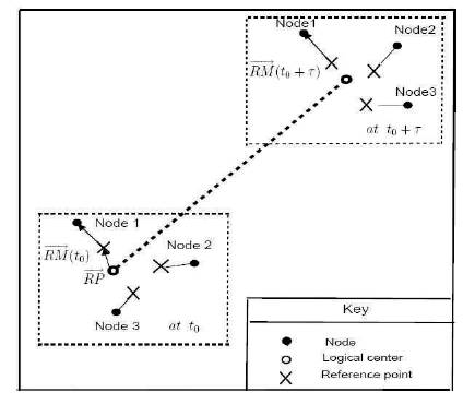
Figure 4. Description of RPGM model

At times t₀ and t₀ + τ the trajectory of the group is illustrated  by superimposing the position of the nodes, their associated reference points and the group's logical center, over time, on the same diagram.

For the purpose of clarity, only the vectors associated with Node  1 have been labeled. It is useful at this point to recall that the for a particular node remains constant throughout time.

1.4 Mobility discussion

Figures 1, 2 and 3 illustrate the typical patterns of travel of a mobile node (s) in models of RPP, RGM, and RPGM, respectively. More space between the dots indicate that higher speeds are involved.

The RRP model has a higher spatial node distribution at the center of the network than near the boundaries [2], while the RGM model has a relatively uniform spatial node distribution across the network.

Moving at the same speed, an RRP node will travel farther than an RGM node over the same time interval, due to the travelling pattern. Figure 3 illustrates a group of three nodes in the RPGM model with the logical center moving according to the RRP model. Also shown is the trajectory of the logical center of the group.

1.5 Incorporation of Mobility Models in Real Life Ad-hoc Applications

Table 1 illustrates impact of these above discussed models in real life scenarios.

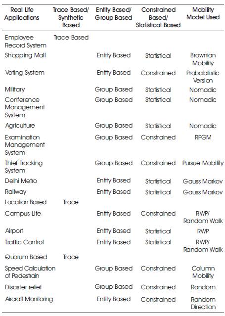
Table 1. Mobility Models in Real life Applications

1.6 Location Management

Location management[16] schemes allow mobile adhoc sources of S for the location of any destination D. In this approach, the node information is stored and updated periodically. Managing location information of the nodes routing protocol is a tedious task. Quorum based and hash-based methods are more accessible in this scheme [17] has suggested uniform quorum systems for effective mobility management in terms of reliability rather than sharing resources. Because the network topology dynamic nature, less infrastructure ad-hoc networks, the calculation of the position of the node is more difficult for static or fixed networks. Consequently, the network layer mobility management is another problem in ad-hoc network.

The objective of this essay is to study the effect of mobility on the performance of an ad hoc network, where nodes have a built-in incentive to collaborate. In this section we return to the original topology considered in Figure 5, where the node N is mobile and follows the path shown in 1 the Figure 6, through the geological centered of the static network.

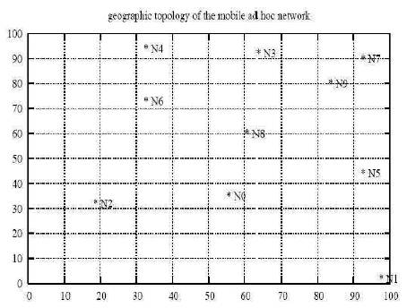
Figure 5. Topology of the mobile ad- hoc network

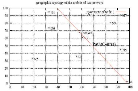
Figure 6. Path of node N1 through the network

Node N₁ moves across the networks and reaches the other edge of the network by the end of the simulation  after 10⁵ seconds of simulation time. To reach this final  location node N₁ moves with a velocity of {-57 x 10^-5 , 98 x 10^-5 ) m/s/

When node N₁ approaches the networks center, it will be  used more frequently as a transit node to carry traffic between other nodes. This can be observed from Figures 7 and 8, which show the bandwidth and power price of node N increase when it is near the center. At the same  time, other nodes have a choice to send traffic through either N₁ or N₈ .

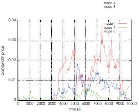
Figure 7. Bandwidth price of the mobile node N1, and two stationary nodes N4 and N8

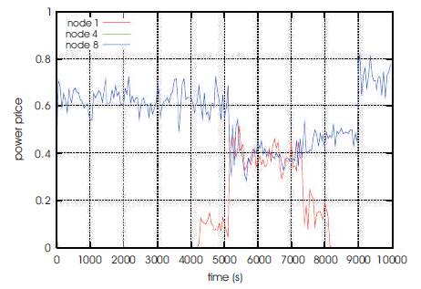
Figure 8. Power price of the mobile node N1, and two stationary nodes N4 and N8

Node N₁ affects the power price of node N₈ ; but helps to reduce it. As node N₁ moves away from the center of the network, these effects on the node power and reduce the price of bandwidth.

The increase in prices associated with the node N1, when you are near the center of the network, and increased traffic load is transmitted to other nodes, it means that your credit balance is also growing, as shown in Figure 9. This increases the capacity of the node N1 to generate traffic, and their willingness to pay is related to your credit balance. Consequently, total production increases, and we see in Figure 10.

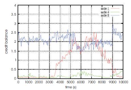
Figure 9. Credit balance of the mobile node N1, and two stationary nodes N4 and N8

Figure 10. Total throughput and total credit

The price increase performance and bandwidth, when the node is close to another node, is also observed when N1 moves away from the center of the network node N1 and near. A comparison of Figure 5 and 10 indicates that the overall performance increases total network N1 to the node moves to the center of this network. In comparison, when N1 moves away from the center out, the general overall performance decreases.

Thus, the results suggest ways in which the overall performance varies with the geological distribution of current users. On the other hand, mobile users can influence not only their own performance, but also the overall network performance.

Mobility management are analyzed and discussed in this proposed work. In addition, models of mobility management in ad-hoc networks are classified. Classification of the mobility model is illustrated on the basis of the entity and the mobility model based on the group. Besides this, the traffic pattern of mobile nodes can be generated through the use of simulators AnSim. AnSim provides good platform to track the movement of the node to change the pause time and speed of the node. The final part of the simulation allows all nodes move independently, and shows that the energy price falls to zero and increases overall system performance when all nodes are near the center of the network.