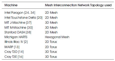
Table 1. Sample commercial and experimental mesh machines.
Multi-Computer Systems (MCSs) are efficient in solving computing-intensive problems. A MCS consists of a number of Processing Elements (PEs) and an Interconnection Network (IN). A fault in any PE and/or the IN can lead to losses in sensitive data and/or the overall throughput. In this paper, the author provide a review of the fault tolerance and reliability assessing techniques of mesh MCSs. A number of fault-tolerant routing techniques are analyzed including the dimension ordering, the turn model, and the block-fault model [52]. In reliability analysis, he considers the sub-mesh reliability exact and approximate models and the task-based reliability computation [8]. It is expected that some of the techniques and algorithms covered in this paper can have applications in the domain of wireless mesh networks.
Multi-Computer Systems (MCSs) include the shared – memory (also known as multiprocessors) and distributed – memory (also known as multi-computers) [41]. Mesh interconnection networks are simple, regular, and scalable [15,55]. A number of computation-intensive Scientific/ Engineering applications can be efficiently solved using mesh-based MCSs. Sample commercial and experimental mesh-based MCSs are shown in Table 1 [13,14, 16, 20, 24, 30, 34, 37, 38].
A MCS is said to be fault-tolerant if it can continue to perform its assigned task(s) in the presence of faulty nodes and/or links [19]. It is possible to achieve fault tolerance in a multi-computer system by using various forms of hardware [31], software, information, and time redundancy. In particular, hardware and software redundancy techniques represent the two frequently used techniques. In this paper, the author focus on fault tolerance and reliability analysis of mesh multi-computer interconnection networks [26, 46, 58].
Definition 1: An n-dimensional mesh is defined as the interconnection structure that has K0 × … × Kn-1 nodes where n is the number of dimensions of the network, and Ki is the radix of dimension i. Each node, i, is identified by an n-coordinate vector (α0, α1, ...αn-1) where 0 ≤ ai ≤ Ki-1. Figure1 shows a 3×3×2 mesh network.
Definition 2: The failure rate of a system, λ, is defined as the expected number of failures of the system per unit time.
Definition 3: The Reliability of a system, R(t), is defined as the conditional probability that the system operates correctly throughout a time interval [t0, t] given that it was operating correctly at t0.
The exponential function R(t) = e-λt can be used to represent the reliability of digital systems. The dimension-ordering Routing (DOR) technique has been used as the basic non-fault-tolerant routing technique in meshes. According to the DOR technique, a message is routed along one dimension at a time in a strict monotonic order on the dimensions traversed. Consider, for example, a 2D mesh network. In this case, messages are routed first along the X-axis and then along the Y-axis. In other words, at most one turn is allowed, namely from X to Y. The DOR algorithm works as follows: Assume that the source node S has dimension (Sx, Sy) and that the destination node D has dimension (dx, dy). The difference in dimension is denoted as (wx = dx - sx, wy = dy - sy ) Wormhole routing is used in routing messages [25, 57]. In other words, a message advances immediately from the incoming to the outgoing channels, given that an outgoing channel is available. Packets are divided into flits (flow control digits) for transmission. The header flit governs the routes, i.e., as it advances along a specific route, the remaining flits follow in a pipelined fashion. According to the DOR the two flits wx and wy are placed respectively in the first two flits of the message. When the first flit arrives at a node, it is either incremented, if it is less than 0, or decremented, if it is greater than 0. If the result of this operation is not equal to 0, then the message is forwarded in the same dimension and direction in which it arrived. However, if the result is 0 and the message arrived on the Y dimension, the packet is delivered to the local node. If, on the other hand, the result is equal to 0 and the packet arrived on the X dimension, the flit is discarded and the next flit is examined upon arrival. If that flit is 0, the packet is delivered to the local node; otherwise, the packet is forwarded in the Y dimension [36]. The X-Y routing has conventionally been referred to as e-cube routing.
Fault-tolerant routing techniques in meshes are introduced below.
The techniques reported in the literature for fault tolerance in mesh interconnection networks can be classified into three main categories [29]. The first category is concerned with fault-tolerant routing algorithms in mesh networks [9, 45]. The second category is concerned with processor allocation schemes for finding a subset of nodes of a given size in the network such that all nodes in the subset are non-faulty [28, 56]. The third category concentrates on ways for providing communications among non-faulty nodes in faulty mesh networks [44]. The author has provided a detailed taxonomy of the fault-tolerant routing techniques in meshes [3, 4]. According to this taxonomy we have classified routing techniques as progressive versus backtracking, minimal versus non-minimal, completely versus partially adaptive [49,51,53]. A progressive routing technique moves messages forward and provides limited ability to backtrack from a node once such node has been reached. A backtracking routing technique searches a network systematically, backtracking as necessary. A minimal routing technique considers only profitable links in making routing decisions at a given node. A non-minimal routing technique considers both profitable and non-profitable links in outing messages. A profitable link is one that always moves a message closer to its destination. A completely adaptive routing technique uses all paths in its class (if profitable, then all profitable links are selected) [42]. A partially adaptive routing technique allows messages to follow both shortest and non-shortest paths in reaching their destinations [3,4].
Table 1. Sample commercial and experimental mesh machines.
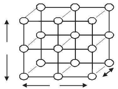
Figure 1. A 3x3x2 Mesh Network
The fundamental concept used in the turn model is to prohibit the smallest number of turns in order to prevent cycles from taking place while routing [12, 22, 50]. Figure 2(a) shows eight possible turns in a 2D mesh network.
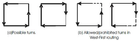
Figure 2. Possible turns in a 2D mesh
As can be seen, in order to prevent cycles in 2D meshes one need to prohibit two of the eight turns. If the two turns to the west are prohibited, the corresponding routing technique is called west-first routing. This is because a given message has to start in the west bound, if necessary, at the source node and then adaptively move south, east, and north [32]. Figure 2(b) shows the six turns allowed (solid lines) and the two turns prohibited (dashed lines) in the case of west first routing in a 2D mesh. Similar routing techniques, e.g., north-last, and negative-first can be found in [32]. Figure 3 shows three examples (Source S1 to destination D1, S2 to D2, and S3 to D3) routing of messages using the west-first routing algorithm under the link fault model in a 2D mesh. As can be seen in Figure 3 the path followed between a source and a destination node is not minima in terms of the number of hops (links) traversed. It should be noted that there are faulty cases under which routing may not be possible under the turn model. The case of messages sent from source node S4 to destination node D4 in Figure 3 is one such case. It should also be noted that because cycles are eliminated, the west – first routing is deadlock-free.
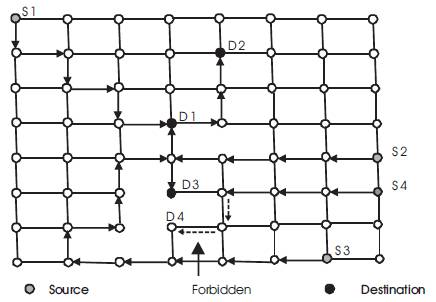
Figure 3. Four west-first routing examples in an 8×8 2D mesh
According to this technique, nodes which cause routing difficulties are identified (labeled). The Node labeling strategy is based on the following two rules [7,9].
The technique starts by applying the NDR to transform faulty regions to rectangular regions. The algorithm then proceeds by applying the NAR in order to activate deactivated nodes residing at the boundaries of faulty regions. It should be noted that the technique may require repetitive application of the NDR. Figure 4 demonstrates the application of the node labeling scheme and the routing of a message around the faulty regions in order to reach the destination. It should be noted that only node fault model is assumed in Figure 4 (links are assumed to be perfect).
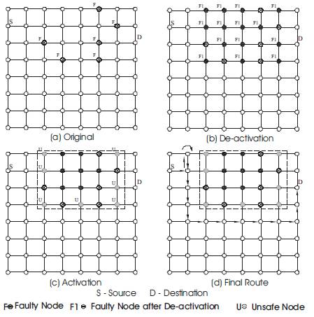
Figure 4. Node labeling routing example in an 8×8 2D mesh
In a mesh network, faults can be of two types: node or link. A third hybrid fault type, called block fault, arises from a combination of both types. According to this model, each fault is assumed to belong to exactly one fault block [39, 43]. A set F of faulty nodes and links is said to form a rectangular fault block, or f – region, if there is a minimum size rectangle connecting various nodes of the mesh such that:
For each f-region in a network with faults, it is feasible to connect the fault free components around the region to form a ring or chain. The faulty ring or f-ring of a given region consists of the fault-free nodes and links that are adjacent (row-wise, column-wise or diagonally) to one or more components of the fault region. An f-chain is formed from connected fault-free components around fault region that touches one or more boundaries of the network. A set of fault rings is said to overlap if they share one or more healthy links. Figure 5 illustrates the concepts of f-ring and f-chain.
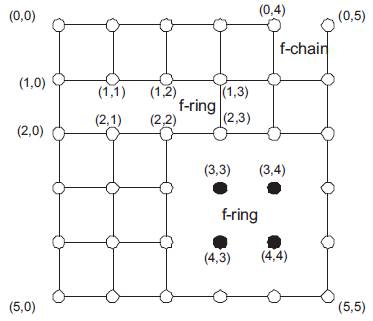
Figure 5. A 2-D mesh with two f-rings and one f-chain
In this figure, there are two f-rings associated with the two rectangular blocks: {(3, 3), (3, 4), (4, 3), (4, 4)}and {<(1, 1), (1, 2)>,<(2, 1), (2, 2)>}and a f-chain associated with rectangular block: {<(0, 4), (0, 5)>}.
The f-cube routing algorithm has been introduced in order to overcome the limitation of the e-cube (see Section 1) in routing messages in faulty meshes. The algorithm uses extra virtual channels to provide fault-tolerant deadlock-free routing based on the e-cube algorithm. A number of f-cube routing algorithms have been introduced. Among these the f-cube2 and the f-cube4 were introduced in [6, 40,45, 47 ]. The f-cube2 algorithm uses two virtual channels (virtual channel c0 is used by row messages, EW or WE, while virtual channel c1 is used by column messages, NS or SN) while the f-cube4 uses four virtual channels (c0 is used for WE, c1 is used for EW, c2 is used for NS and c3 is used for SN). The f-cube2 algorithm can tolerate non-overlapping faulty blocks, in cases where there is no shared links between multiple fault rings. The algorithm follows the e-cube routing unless misrouting is needed. Misrouting is performed if the next e-cube hop is blocked due to the existence of a faulty component (node and/or link) on the path from the source to the destination. Misrouting in f-cube2 is indicated via a status parameter. Once a message, M, is misrouted then its status is changed from normal to misrouted and proceeds according to the Set-Direction(M) procedure shown in Figure 6 [27]. It is assumed that the message M in Figure 6 is currently hosted at node (a1, a0) and that the destination of the message is node (b1, b0) Figure 7 shows an example of f-cube2 routing in which the source node is (1, 0) and the destination node is (4, 4).
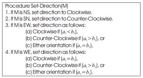
Figure 6. The Set-Direction procedure for misrouting in f-cube2
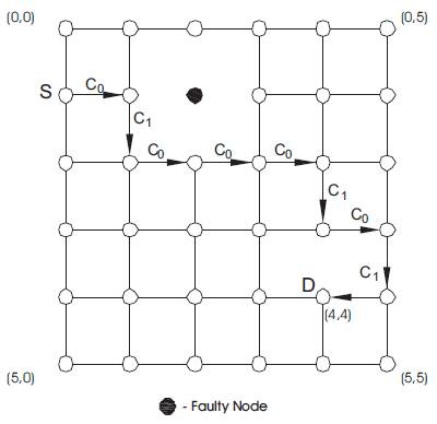
Figure 7. Example f-cube2 routing in a 2D mesh
The f-cube4 algorithm has been introduced as an extension to the f-cube2 algorithm. According to this algorithm, it is suggested to route messages on overlapping f-rings and f-chains. The f-cube4 algorithm uses four virtual channels, c0 ,c1 ,c2 ,c3 ,such that WE messages use c0, EW messages use c1, NS messages use c2, and SN messages use c3 channels. This routing algorithm can tolerate overlapping fault blocks, i.e. a set of fault rings that share one or more healthy links [48]. Similar to f-cube2, the f-cube4 routing algorithm routes all messages according to the e-cube algorithm unless misrouting is needed. If a message is blocked, it is misrouted according to the following procedure:
Figure 8 shows an example of f-cube4 routing on two overlapping f-rings and one f-chain in a 2D mesh.
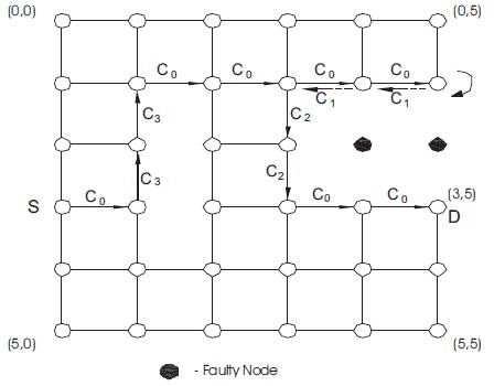
Figure 8. Illustration of f-cube4 routing on f-rings and f-chains in a 2D mesh
Subsequently, the f-cube3 algorithm has been introduced as an improved version of f-cube4 algorithm, where only three virtual channels (c0 ,c1 and c2) ,per physical channels are used. According to the f-cube3 routing algorithm, a given message starts as a row message and its direction is set to null. If not blocked by faults, the message is routed along its e-cube hop. Being a row message and if a0= b0 then the message type is set to NS (SN), if a1> b1 (a1< b1). When faults are encountered then the direction of the message is changed depending on the message type as follows assuming that the message is currently at node a1 , a0 and its destination is node b1 , b0:
Figure 9 shows an example for f-cube3 in a 2D mesh between source node S (5,0) and destination node D (1,2) [45].
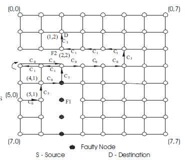
Figure 9. Example f-cube3 routing in a 2D mesh
This routing algorithm is based on the turn model [21] presented above. The algorithm splits any physical channel into four virtual channels. Five sets of virtual channels were identified. The first two sets (the basic sets) are used to provide deadlock-free non-minimal [54], fully adaptive routing [35]. The second set consists of two virtual channels and is used to tolerate faults occurring in the east and the west borders. The last set is a pool of virtual channels that can be used by all the messages. The routing algorithms used in the basic sets are west-last (route a packet first adaptively north, south, east, and lastly west) and east-last (route a packet first adaptively north, south, west, and lastly east), respectively to prevent deadlock involving the X direction channels. The algorithm allows 180 degrees turns except in the X direction channels. Dimension-ordered routing is used in east (west) border to prevent deadlocks not involving X direction channels. Figure 10 shows examples of these algorithms with routing paths in case of link and node failures [2].
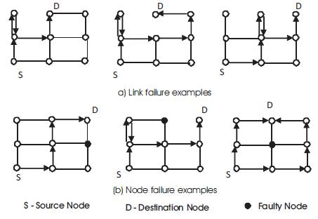
Figure 10. Virtual-Channel -based Turn Routing in 2D Mesh
The author have conducted a survey and comparison of routing techniques in mesh networks in [3]. Table 2 summarizes the main characteristics of a number of these routing techniques. The table shows the fault model and the properties of the technique used. These properties include minimality (in terms of the number of links traversed before arriving at the destination node), adaptivity (ability of the algorithm to backtrack whenever arriving at a deadlock point along the route), and the dimensionality (mesh dimension that can be supported by the algorithm). As can be seen, among the four techniques presented, the turn model is the only one that achieves minimality. However, the node labeling and the block fault models are fully adaptive as compared to the limited adaptivity of the turn model. The node labeling and the block fault model techniques tradeoff minimality for adaptivity. While the dimension ordering model is the least among the four techniques in terms of minimality and adaptivity, it is the only one that, guarantees deadlock-free routing of messages.
The issues related to reliability analysis of meshes are introduced next [5]. It should be noted that the most commonly used measure for reliability of mesh-connected multi-computer network is Submesh Reliability (SR) [33]. According to the SR measure, a system is considered working as long as some minimum-size submesh is functional. The SR measure is particularly useful in meshes due to the possibility of executing a given algorithm on a number of meshes of size.
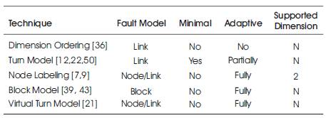
Table 2. Main properties of a number of fault-tolerant mesh routing techniques
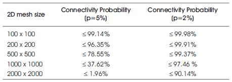
Table 3. The connectivity probability for 2D meshes
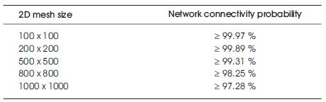
Table 4. 2D mesh connectivity probability for various network sizes and p = 2%
A simple approach in dealing with the connectivity of a given mesh network in the presence of node failure is to divide the network into a number of smaller k-sub-meshes such that each k-sub-mesh has a given degree of connectivity. If all k-sub-meshes are shown to be connected and each k-sub-mesh is shown to be connected i.e., its non-faulty nodes are connected, then the entire mesh is considered to be connected. The advantage of such approach is to reduce the problem of dealing with the connectivity of the entire mesh network into that of determining the connectivity of smaller sub-meshes. Calculating the probability of k-sub-mesh connectivity for each smaller k-sub-mesh can be made either through exhaustive enumeration or through simple combinatorial analysis [10].
Consider the case of a 2D mesh network of size M x N (M is the number of rows and N is the number of columns). Each node in such 2D mesh is given a pair of coordinates (x, y), where 1≤ x ≤ M & 1≤ y ≤ N. A pair of nodes v vx, vy and u ux, uy are said to be neighbor if 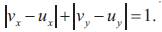
It has been shown in [27] that in a 2D m x n mesh, where m , n ≤ 3 if each node fails independently with a probability p> 0 then an upper bound on the probability that the 2D mesh is connected is given by:
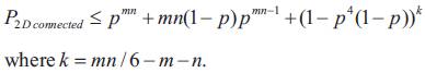
Consider, for example, the case of having node failure probability p = 5% and p = 2%, respectively, Table 3 shows the results obtained using the above bound for various network sizes. The table shows that the 2D mesh network connectivity probability drops substantially as the size of the network increases, given a low node failure probability. For example, a network connectivity probability drops to almost 2% when the network size reaches 2000 × 2000 for p = 5%. This indicates that it is necessary to control the node failure probability in such a way such that high connectivity probability for large size mesh networks can be achieved.
In the following discussion and without loss of generality, it will be assumed that the dimensions, M and N of the entire mesh are divisible by some integer value, k.
Definition 4: define a k-sub-mesh as a square mesh having k2 nodes and whose borders are determined by two integers a and b such that 0 ≤ a < (M/k) -1 & 0 ≤ b < (N/k) -1, where ak+1≤x≤ (a+1) k and (x, y) represents the coordinates of nodes in each sub-mesh.
Definition 5: A given 2D mesh network of size k x k is said to be k-sub-mesh connected if the non-faulty nodes in the network form a connected graph and that each side of the k-sub-mesh contains more than k/2 non-faulty nodes.
Assuming that each node in a 2D mesh k x k fails independently with probability p, then the probability of such network being k-sub-mesh connected can be calculated as: 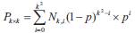 were Nk,i is the number of ways in which i nodes can be removed from the k x k mesh such that the remaining nodes form a connected graph and each side of the k x k mesh has more than k/2 nodes.
Definition 6: A given 2D network of size M x N where M > k and N > k, is said to be k-sub-mesh connected if and only if all of its k-sub-meshes are k-sub-mesh connected.
The probability of a 2D mesh of size M x N being k-sub-mesh connected given that all of its k-sub-meshes are k-sub-mesh connected is bounded by PMxN ≥ (Pkxk) MxN/k2 . Table 4 shows the bonds on network connectivity probability for various mesh sizes when node failure probability is p = 2% and assuming 10-submesh connected of 10×10sub-meshes.
Comparing the results obtained in Table 4 with those obtained in Table 3, it is clear that in order to achieve 2D mesh connectivity around the 99% level using the k-sub-mesh connectivity model it is required to bound the node failure probability by 2%.
In this approach, the probability of executing a task that requires a fault-free mesh of size m x n in a mesh of size M x N where m ≤ M and n ≤ N is computed. Computation of such probability can be performed in three steps [1, 17, 18, 23].
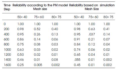
Table 5. Reliability Figures using PM model and simulation
Step 1: In the first step, the probability of finding at least n consecutive functioning nodes in a single row is computed. Finding at least n consecutive functioning nodes in a row having N nodes can be computed using the following recursive expression:
where 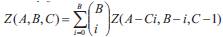 denotes the number of ways in which A identical objects can be placed in B boxes such that each box has at most C objects and R(t) = e-λt is the reliability of a node.
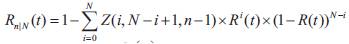
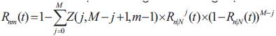
Step 2: In the second step, the reliability of at least m consecutive components is computed where each component is a functional row. A row is considered to be functional if at least n consecutive nodes are working (Step 1 above). The reliability of a row Rn/N(t) becomes the reliability of each of the M component in the vertical line. This can be computed using the following expression:
Step 3: This step is to ensure the alignment of the working nodes to form an (m×n) mesh. It has been shown that the probability of such alignment is extremely difficult to compute. Therefore an approximate approach is used. This approach states that if there are at least m consecutive rows each having  consecutive working components, then a working (m×n) mesh can be obtained irrespective of the alignment of components.
The method presented in [17] is based on the principle of inclusion and exclusion in arriving at approximate expression for sub-mesh reliability in 2-dimensional meshes using a constant computational complexity. According to this model, called the Partitioned Mesh (PM) model, a mesh is divided into non-overlapping partitions. Partitioning can be made row-wise (RP) or column wise (CP). According to RP, an M x N mesh can be partitioned into  where 2n ≤ N. While according to the CP, an M x N mesh can be partitioned into
  where 2m ≤ N.
The sub-mesh reliability is approximated as a polynomial with only two terms such that RRP (t) = X x Rmn (t) - (X-1) x Rmn+m (t), where X is the number of possible locations for the mesh of the required size (m × n) and Rmn (t) is the probability of having a mesh of size m × n at any specific location. Approximating the entire mesh as consisting of S RP meshes connected in parallel, then the system reliability is modeled as Rsys (t) = 1-(1- RRP (t))s. Similar expression can be derived using the CP model. We have compared the results obtained using the PM model with those obtained using simulation [17, 18, 24] for a mesh size of (100 x 80) and with three mesh sizes: 50 x 40, 75 x 60, and 80 x 75 (with λ= 0.000001). See Table 5.
As can be seen from the table, for low degradation such as in the cases 75 x 60, and 80 x 75 the analytical model produces close results compared to those produced by simulation model. At higher degradation such as in the case 50 x 40 the analytical model produces inferior results and in particular as the system reliability falls down.
In this paper, the author provided a review of the techniques used to achieve fault tolerance and reliability in mesh multi-computer networks. We covered the dimension ordering routing model, the turn model, the node labeling model, and the block fault model. The paper has also covered the sub-mesh and task-based reliability analysis of mesh networks. Examples showing the application of those techniques have also been provided. The paper provides designers of mesh networks with the criteria needed to assess the reliability and fault tolerance of their designs. The paper also shows designers the different methods that can be used to analyze and enhance the fault tolerance and reliability and aspects of existing conventional interconnection networks using mesh systems.