The wavelet networks (wavenets) is an approach for system identification in which nonlinear functions are approximated as the superposition of dilated and translated versions of a single function, which is localized both in the time and frequency domains [1,2]. Given a sufficiently large number of network elements (called “wavelets”), any square-integrable function can be approximated to arbitrary precision [3]. The following are the advantages of Wavenet over similar architectures [4]:

(i) Unlike the sigmoidal functions used in neural networks of the multilayer perceptron type, wavelets are specially localized. As a result, training algorithms for wavelet networks typically converge in a smaller number of iterations when compared to multilayer perceptrons.

(ii) The magnitude of each coefficient in a wavenet can be related to the local frequency content of the function being approximated. Thus, more parsimonious architectures can be achieved, by preventing the unnecessary assignment of wavelets to regions where the function varies slowly. This property is not shared by networks of conventional radial basis functions (Gaussians).

(iii) It is not difficult to add or delete the hidden units by not affecting the performances because the basis function is localized in time-frequency plane.

The term “wavelet” as it implies means a little wave. This little wave must have at least a minimum oscillation and a fast decay to zero, in both the positive and negative directions, of its amplitude [5]. Wavelets are a powerful tool for function analysis and synthesis. To begin the discussion, a brief introduction to the continuous wavelet transform and inverse wavelet transform will be given. Following this, a comparison with Fourier analysis will be presented to highlight the strengths of wavelet theory. The environments being considered will result in functions dependent on state (position) as opposed to time. Therefore, the domains of interest will be space-frequency as opposed to time-frequency. This section concludes with a discussion on discrete implementations of the inverse wavelet transform, which is the form used in the wavelet network (wavenet) [6].

1.1 Continuous Wavelet Transform

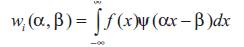
The continuous wavelet transform (CWT) can be expressed as follows:

(1)

The parameter ‘?’ controls the width (dilation) of the wavelet, while ‘?’ controls the position (translation). The variable ‘?’ is a family of functions based on a single analyzing wavelet, along with its translated and dilated versions. The result of this transform is a set of wavelet coefficients, ranging over different widths of wavelets, called levels. The translation parameter is adjusted according to the dilation parameter to ensure that the entire operating range is covered. As an example of what a family of analyzing wavelets would look like, consider the Mexican hat (second derivative of the Gaussian) wavelet shown in Figure 1.

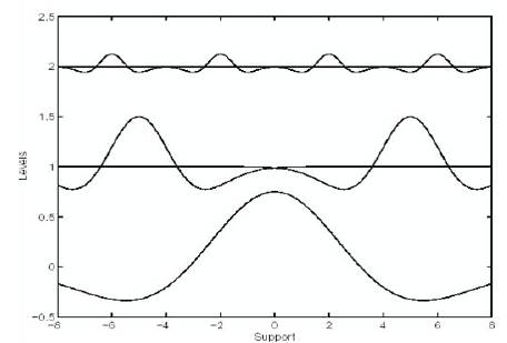
Figure 1. A conceptual view of how the wavelet transform works using a Mexican hat wavelet

The wavelet transform analyzes a function at different wavelet levels. A wavelet level is defined as a set of translated wavelet with constant dilation. Wavelets have been compared to microscopes with the ability to zoom in on short lived high frequency features. This fact can be noted by observing that as the wavelet becomes more contracted, it approaches a discontinuity. Using more levels in the analysis results in the ability to extract more detailed (high frequency) features.

Of greater interest to this work is how to use wavelet theory to reconstruct functions. This is achieved by applying the inverse wavelet transform:

(2)

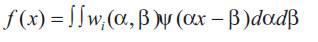
Which states that a function can be reconstructed by summing over the entire range of translated and dilated wavelets [6].

1.2 Wavelet and Fourier Analysis

Fourier analysis shows that any periodic function can be represented by the sum of sines and cosines. Similarly, wavelet theory shows that an arbitrary function can be represented by the sum of wavelets. The following points regarding the wavelet theory will be highlighted:

? Wavelets are capable of representing functions that are choppy, discontinuous, and potentially nonperiodic.

?The wavelet transform represents the function in both space and scale (frequency), while the Fourier transforms addresses frequency alone.

An advance in Fourier analysis provides a method to represent a function in both space and frequency. The concept is referred to as the short time Fourier transform (STFT). The basic approach is to fix a window size of constant length, and change the frequency within the window using a finite section of a sine or cosine function. Once the window size has been defined it remains constant throughout the entire space-frequency plane. Although the approach is sensible, it suffers from the issue of defining window size. If the window is large then low frequency content is captured but it becomes difficult to pinpoint the location of high-frequency features. If the window size is small then high frequency features are captured with good accuracy, however the lowfrequency content is missed. Based on the above notion, it would be nice if both large and small windows could be used. This is precisely what wavelet theory provides. Wavelets automatically adjust the size of the window, through the dilation parameter, to compensate for high and low frequency content.

The above comparison was a brief introduction into the differences between Fourier and wavelet analysis. The intent was to introduce some characteristics inherent to wavelet analysis that make it a powerful tool when applied to nonlinear functions. For a full and detailed comparison between Fourier and wavelet theory, the reader is referred to [7].

1.3 Discretization Methods

Since the functions of interest to this work will always consist of data points sampled at a constant time step, it is appropriate to obtain a discretized version of the inverse wavelet transform (2). There are various methods for obtaining a discretized version of (2). The general structure for the inverse discrete wavelet transform is as follows:

(3)

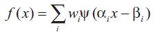
For stable reconstruction of the function, the above form must meet certain criteria. One common way is to construct a family of wavelets that constitute an orthonormal basis. Another method is to create a family of wavelets that constitute a frame [6].

1.4 Wavelet Frame

Two categories of wavelet functions, namely, orthogonal wavelets and wavelet frames, were developed separately by different groups. Orthogonal wavelet decomposition is usually associated to the theory of multiresolution analysis [8]. The fact that orthogonal wavelets cannot be expressed in closed form is a serious drawback for their application to function approximation and process modeling. Conversely, wavelet frames are constructed by simple operations of translation and dilation of a single fixed function called the mother wavelet, which must satisfy conditions that are less stringent than orthogonality conditions [9].

To constitute a frame, the discrete wavelet transform generated by sampling the wavelet parameters (time/frequency) on a grid or lattice, which is not equally spaced (unlike the short-time Fourier transform, STFT), must satisfy the admissibility condition and the lattice points must be sufficiently close to satisfy basic informationtheoretic needs [5].

A daughter wavelet ?_i(x) is derived from its mother wavelet ?(x) by the relation:

(4)

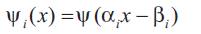
Where, (?_i) represents translation factor and (?_i) dilation factor [9].

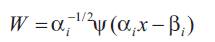
The family of functions generated by (?) can be defined as:

(5)

A family of wavelets is called a frame if the energy of the wavelet coefficients (sum of their squared moduli), relative to the signal, lies between two positive constants A and B (A>0 and B < ? ), called frame bounds.

(6)

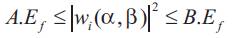
Where, is defined to be the energy of the function to be identified. If a family of functions satisfies the above expression then it automatically passes the admissibility condition [10].

The similarity between the inverse wavelet transform and the neural network motivates the use of a single layer feedforward network [6].

A wavenet, as shown in Figure 2, is a neural network with two layers whose output nodes form a linear combination of wavelet basis functions that are calculated in the hidden layer of the network. The basis used in wavenet has been given the name “wavelons”. These wavelons produce a localized response for an input impulse. That is, they produce a non-zero output when the input lies within a small area of the input space [11].

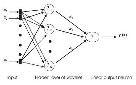
Figure 2. Feed forward Wavelet Network (wavenet)

The hidden neuron activation functions (wavelons) are wavelet functions [12]. There are two commonly used types of activation functions: global and local. Global activation functions are active over a large range of input values and provide a global approximation to the empirical data. Local activation functions are active only in the immediate vicinity of the given input value [13].

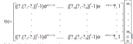
From the above model, the wavenet has the following form:

(7)

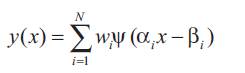
Where,

?The parameter (w_i), is a weight parameter between the hidden layer and the output unit (wavelet coefficient).

?The parameter (?_i) and (?_i ), are the dilation and  the translation parameter respectively.

?The parameter (N) is the number of wavelons

?Where (n) is the number of input samples.

2.1 Final Model

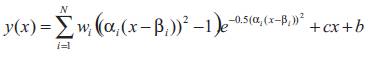
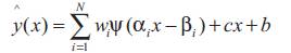
The identification process will be applied to a class of environments that typically exhibit linear regions along with the nonlinearities. In order to produce a result that captures both of these aspects [6], additional connections are made directly from input to the output neurons, as shown in Figure 3. The final model takes the form [12]:

(8)

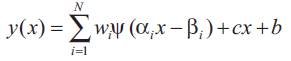
Where, parameter (c) and (b) are the linear coefficients and bias term respectively and (N) is the number of wavelons in the network.

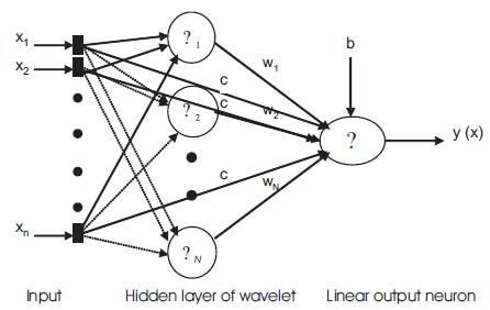
Figure 3. Feed forward Wavelet Network (wavenet) with Direct connections

The wavelet family, which constitutes a frame, consists of the mother wavelet (Mexican hat wavelet) located at the origin along with its translated and dilated versions.

(9)

The following matrix of size n x (N+2) will be defined for use in the function (9).

(10)

2.2 Initializing Wavenets

Due to the fact that wavelets are rapidly vanishing functions [9], the following should be noted:

?A wavelet may be too local if its dilation parameter is too small.

?It may sit out of the domain of interest if the translation parameter is not chosen appropriately.

The initial set of wavelets is determined from the input data and the desired resolution. The desired resolution corresponds to the number of wavelet levels which are defined on a dyadic grid [6].

The input vector is pre-processed component-wise using the following expression:

(11)

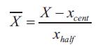
Where,

(12)

(13)

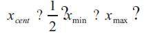
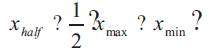
For the duration of the section a bar above a variable denotes pre-processed data. The idea behind choosing wavelets for the frame is to construct a pyramid that grows upward with increasing dilation. Based on the range of input data and specified number of levels the wavelets are scanned to obtain the translation and dilation parameters.

(14)

The variable level corresponds to wavelet level, that in practice usually four or five levels is sufficient. Using a dyadic grid for the wavelet levels, the first dilation parameter is, (dilation=2^o =1). The mother wavelet, centered at the origin (?=0) with dilation parameter (?=1), is always included in the truncated frame.

Therefore, the truncated frame consists of the following wavelets:

(15)

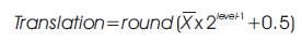
To add the translation parameter, its value is modified to ensure that it covers the entire operating range. This is accomplished using the following relationship:

(16)

The process continues through (m ) wavelet levels with a final dilation value of (dilation=2^m ). As the dilation parameter gets large, the wavelet becomes more contracted and will only be included if the input data exhibits high frequency characteristics.

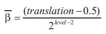
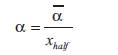
To complete the process, the translation and dilation parameters are post-processed using the following equations to obtain the final set of wavelet parameters:

(17)

(18)

In this section, an algorithm to design wavenets using genetic algorithms is proposed. The rough flow of this algorithm is as follows.

The proposed GA for training wavenet can be summarized as follows:

Step(1): Initialize translation and dilation parameters of all hidden wavelon and create an initial population of chromosomes and set current population to this initial population. Initialize crossover rate (Pc), mutation rate (Pm), and population size (N). Chromosome contains weights (w), linear coefficients (c) and bias (b).

Step(2): Approximates any desired signal by:

(19)

Step(3):Compute the sum square error (SSE) for all chromosmes, SSE is equal to the differences between target class number and the calculated class number. Thus by denoting,

(20)

by a time-varying error function at time , where (x) is the desired response. The energy function is defined by

(21)

Step(4):Evaluation, where each chromosome is evaluated according to its value of the fitness function.

(22)

Step(5):Save best population (beginning of elitism technique).

Step(6): Selection in which parents for reproduction based on their fitness are selected.

Step(7):Recombination, which generates two offspring from the two parent chromosomes through the exchange of real string (crossover).

Step(8):Mutation, which apply a random mutation to each offspring.

Step(9):Replace old population with new population.

Step(10):Copy best population to the new population in the next generation.

Step(11): Go to step(2), if some criterion is not reached.

Some computer experiments were carried out to evaluate the performances of this method.

4.1 Static Nonlinear Mappings

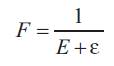
The first example is the approximation of a single variable function, without noise, given by:

(23)

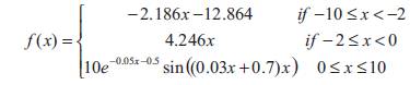
This example was first proposed in [2], which is one of the seminal papers on wavelet networks (wavenets).

The following simulations will describe the results of the wavenet network performance employing Mexican Hat super-mother wavelets. GAs are used for searching an optimal arrangement of the weights. The following parameters are set, population size= 100, crossover probability (Pc)= 0.87, and mutation probability (Pm)= 0.20.

Figure 4 captures the learning performance of the wavenet network using (31) Mexican Hat wavelets at level (5), SSE of 0.0405 is reached for only (47) generations.

4.2 Identification of a Noisy Impulse Corrupted Model

The system y(x) resumed with 10 db SNR (noise ?²=0.1) and an outlier at x = 80.

(24)

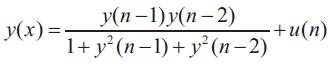
Where u(n) = 0.8 sin (2?n/50) random noise with normal distribution.

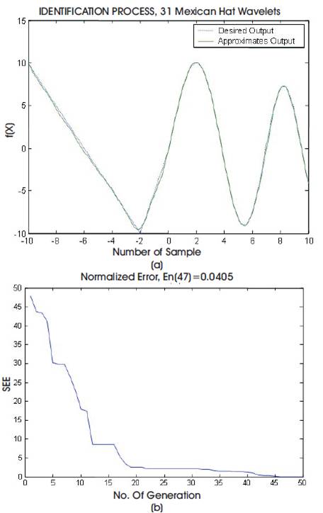
Figure 4. Simulation Results for Static Nonlinear System using GA.

Figure 5 presents the noisy impulse corrupted system data, and the resynthesized system signal using the estimated optimum parameters corresponding to (15) Mexican Hat wavelets. As a result, the network can tolerate some noisy effects and impulse corruption. SSE of 0.3101 is reached for only (38) generations. The following parameters are settings, population size= 100, crossover probability (Pc)= 0.7, and mutation probability (Pm)= 0.2.

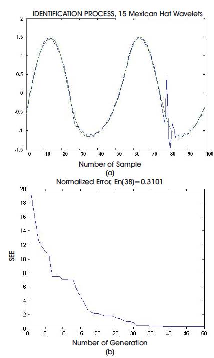
Figures 5. Simulation Results for the Nonlinear Dynamic System Using GA.

The idea of combining wavelet theory with neural networks resulted in a new type of neural network called wavelet networks or wavenets. The wavenets use wavelet functions as hidden neuron activation functions.

The wavenet networks can be used for function approximation to static and dynamic nonlinear inputoutput modeling of processes. The wavenet improves the performance of the trained network for fast convergence, robustness to noise interference, and high complex ability to learn and track of unknown / undefined complex systems

Genetic algorithm has been used successfully for training wavenet because GAs reach quickly the region of the optimal solutions. Tests shows that GA obtain best weight vector and produces a lower sum square error (SSE) in a short period of time (No. of iterations).