With an increasing demand to structure data for efficient access in large data warehouses, hash tables serve as an efficient way for the implementing dictionaries by providing with keys to values of the dictionary. However, such algorithms tend to get computationally expensive due to collisions in a hashing (or hash) table. A searching in the hash table under reasonable assumptions, could take an expected time of O(1) (Aspnes, 2015). Although, in practice, when hashing performs extremely well, it could take as long as a linked list in a worst case scenario, which is O(n) (Sing & Garg, 2009). Collision occurs when two keys hash to the same slot or value. The purpose of this article is to research and provide a comparative study on the different hashing techniques and then implement a suitable one for a banking record system scenario.
A data structure can be defined as a systematic way to store and organize data in a computer system for efficient access, retrieval, deleting, and other similar operations (Srivastava & Srivastava, 2003). One of the basic techniques for the improving algorithms is to structure data in such a way that the resulting operations can be efficiently carried out (Hash Tables, 2016). For example, words can be quickly searched for in a language dictionary. This is because all the words are apathetically sorted. In perspective, a dictionary is organized as a sorted listed of words. It would be almost impossible and impractical to search for millions of words in an unsorted language dictionary.
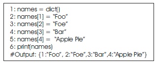
A dictionary, associative array, map, or symbol table is an abstract data type composed of a collection of (key, value) pairs. An example of a dictionary of the authors of this article is given in code snippet 1 as a python program.
Code snippet 1: A dictionary entry
This unique key-value mapping forms the basis of a dictionary. Thus, allowing trivial operations on dictionaries:
A map is a dictionary with no duplicate keys. Henceforth, a map can be defined as the ideal metric for comparing the rate of collision of the dictionaries implemented using hash tables.
Hash values are beneficial in providing examiners with the ability to filter known data files, match data objects across platforms, and prove that data integrity remains intact (Danker, Ayers, & Mislan, 2009). A method and apparatus for performing storage and retrieval in an information storage system is disclosed in (Nemes, 1992) which, uses the hashing technique. A method having index of two parts: a primary index, which facilities data pruning, and a secondary index, which stores the uncertainty information of each object is described in (Rathi, Lu, & Hedrick, 1991) and an extensible hash table is proposed. An overview of geometric hashing and its advantages are discussed in (Wolfson & Rigoutsos, 1997). A semi-supervised hashing framework that minimizes empirical error over the labeled set and an information theoretic regularize over both labeled and unlabeled sets is proposed in (Wang, Kumar, & Chang, 2012). The various hash table techniques are presented in (Devillers & Louchard,1979). It includes the popular techniques like open addressing, coalescent chaining, and separate chaining. A general method of file structuring is proposed in (Coffman & Eve, 1970), which uses a hashing function to define tree structure. Two types of such trees are examined, and their relation to trees studied in the past is explained.
This technique works well only when the key domain is small. Therefore, it is useful for creating smaller databases or using it in programs that refer to a shared variable constantly. Though creating a hash table is tedious and complex, search, insertion, and deletion in this case would only take constant O(1) time as compared to O(n) for an array data structure. Furthermore, both an array and hash table take the same space complexity in the worst-case scenario, which is O(n).
The direct address table comprises of an array, say T, with values T [0, 1, 2, ..., n − 1], where n is not an infinitely large positive integer. Each position (address or sometimes referred to as slot) corresponds to a key for a value. Trivial dictionary operations in direct addressing are given in code snippet 2.
In direct addressing, there is one position for every possible key (index). The direct address table is impractical, when key size is large. e.g. to store the keys 5, 77, 501, 600, and 1088, we need a table of size 1089. Thus, the data can be extremely spread and form clusters of uneven buckets.
Code snippet 2: Dictionary Operations
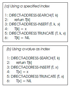
A hash table is an effective alternate to the direct addressing. Rather than using the value as the index itself specifying the index like dictionaries do, a separate array is used to store the keys for each value. The size of the array is proportional to the number of keys used. Since the keys need not necessarily be consecutive in a real-time scenario, the data would not be evenly distributed.
A hash function h(k) is defined to compute the address/position/slot of the element using the key k. In this case, h: N → T[0, 1, 2...n], where n << N or h(k) is the hash value of key k. Since indexes are not necessarily consecutive, hash functions can be designed to reduce the range of array index and prevent clustering or formation of buckets, and allow an even distribution.
However, Hashing may suffer from collisions. The collision occurs when two or more keys hash to same address/slot. Say, for some given keys k8 and k14 map to the same slot, such that h(k8) = h(k14), where h(k) is the hash function. Rate of collision depends primarily on the hash function. Given below are a list of the different hash functions:
1) Division method: Consider an example of a hash table of size, m = 20 using a module function. The hash function in Table 1 is an example of a division method, where the hash function is described using the formula, h(k) = k mod m.
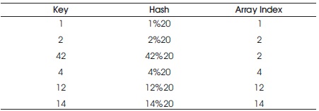
Table 1. Hashing using Division Method
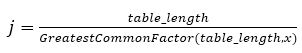
While selecting m, some values such as 2p should be avoided. In this case, h(k) will be the lower order bits of k. A prime number is often a good choice to enable an evenly distributed hash table. Hence, by avoiding clustering of values into a small number of buckets, the hash table will perform more consistently. If in case a composite number is chosen, say a multiple of 2, 3, 4, 5... then the keys would be clustered in j number of clusters or buckets, where,
2) Multiplication Method: The following function can be used to implement the multiplication method, h(k)=[m .(k . A mod 1)], where 0 < A < 1. If key k can fit in a single word of w bit, then corresponding A is chosen of the form s/2w, where 0 < s < 2ω. An example for an optimal choice of A would be the Knuth recommendation Ratio of A = (√5-1)/2.
3) Folding Method: The hash function is defined by the formula:

Here, partitions of the key is done into k1, k2, k3,..., kr, where each part has same number of digits except possibly the last. Then, add these numbers by ignoring carry to generate address.
4) Mid-Square Method: A simple method, where the key is squared, and digits from both ends of k2 are truncated.
The recording system is similar to the one used by banks for tracking their customers. Every customer is provided with a unique identification number or an account number. The data must be uniformly spread, this is not an issue in array as all the elements are stored in one contiguous block of memory. But during hashing, clusters may be formed. An ideal system must be able to overcome this issue over several collisions. Primarily, the rate of collision depends on the hash function. A criteria of a hash function is that given a hash function, h(), it should uniformly distribute the hash address through a structure [0..m], minimizing the number of collisions.
It is almost impossible to avoid collision completely because m << N, where N is the size of key domain. Though hash functions can be designed to minimize the scope of collision, a process for resolving the collisions that occur needs to exist.
In open addressing, no additional elements are stored outside the hash table. To perform insertion, probing is performed on hash table until an empty slot is found for a key. The different types of probing are given below:
1) Linear Probing: Given an original hash function as such, h’ = U → 0, 1, 2, ..., m -1, also called an auxiliary hash function (Cormen, Leiserson, Rivest, & Stein, 2001), linear probing using a hash function of the form:

However, this form of probing suffers from primary clustering. With an increase in the occupied slots, the average search time increases. Therefore, as an empty slot gets filled up and has i slots preceding it, the probability of clustering increases with the equation i + 1/m.
2) Quadratic Probing: Given an original hash function as such, h’ = U → 0, 1, 2, ...., m-1, quadratic probing using a hash function of the form:

where, c1 and c2 are positive auxiliary constants. Quadratic probing is very similar to linear probing, except for the fact that the probing uses a quadratic sequence. For example, a quadratic hash function h’(k)+c2j2 would give equations of the form h+0, h+1, h+4, h+9, h+16,...h+n for probing.
Clustering occurs in quadratic probing only if two keys have the same initial probing value. Since, h (k1, 0) = (k2, 0) ⇒ h (k1, I) = h (k2, I), clustering does occur, but is at a much milder rate. This form of clustering is called secondary clustering (Cormen et al., 2001).
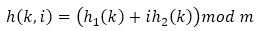
3) Double Hashing: Given an original hash function as such, h1 = U → 0, 1, 2,..., m-1 and another function h2 = U→ 1, 2, 3,..., m. The hash function is of the form:
Double hashing is likely to inherit properties of an 'ideal' scheme of uniform hashing. Rather than using O(n) probe sequences like linear or quadratic probing does, it uses a distinct probe sequence produced by each possible h1(k) and h2(k) pair. Thus, these sequences increase in the order 2 of O(n2), giving it a significant performance improvement. However, the double hashing function is notably harder to design for larger data sets like in a banking system (Cormen et al., 2001).
In chaining, a linked list is maintained for each slot. All the elements that hash to the same slot are placed into the same linked list. For example, a hash-table slot T[i] could contain a linked list of all keys whose hash value is i. For example, h(k1) = h(k4) and h(k5) = h(k2) =h(k7) (Cormen et al., 2001). Collisions can be easily resolved using this method. However, limitations may include searching through extremely long linked lists chains. Hence, the worst-case time for searching is O(n).
Expected value of length of the list is given by α = n/N, where n/N or α is also called the load factor of the hash table, that is, the average number of elements stored in a chain, while n is the number of keys and N is the table size.
An unsuccessful search would yield an average hash time of O(1 + α) under the assumption of uniform hashing in an increasingly long chain. This is because (Cormen et al., 2001), the length of the chain at some T[k], would result in a number of keys in the form n= n1+n2 +n3+,...+nN-1, where k = 0, 1, 2,.... N-1. Thus, giving an average value of nk as n/N = α, since n is the number of keys and N is the total number of elements in the table size.
The decision between the two determines primarily on the cost of the operations being conducted. Both use few probes. However, double hashing is likely to take more time since it requires two hashing functions. It requires O(n2) probe sequences, which means it makes a more efficient use of the memory as compared to linear or quadratic probing in that, where O(n) probe sequences are used (Cormen et al., 2001).
Therefore, though fewer probes are used, it takes more time as the interval between probes is computed by another hash function (Horowitz, Sahni, & Rajasekaran, 2008). This is when a collision occurs when using the first hash function. On the other hand, primary and secondary clustering are avoided, but with the drawback that implementation of double hashing is more complicated than linear or quadratic hashing.
The average run time of a double hashing is given below. In a non-full hash table, assuming no previous removals, the average running time of insert, find, remove is (Vlajic & Natalija, 2003):

Though quadratic and double hashing perform better than linear probing on an average case, they suffer as the table begins to fill up. As this happens, and as α → 1, all open addressing schemes suffer from a linear worst-case time complexity, O(n). Furthermore, quadratic and double hashing share similar performances (Singh & Garg, 2009).
Separate chaining takes the least number of probes and hence is the most efficient for probing. This comes at the cost as separate chaining uses extra memory for links. On the other hand, double hashing also uses extra memory implicitly within the table to terminate probe sequence (Hash Tables, 2016). Lastly, Open-addressed hash tables cannot be used if the data does not have unique keys.
The codes below, were used to calculate time by taken by the INSERT function of the algorithm. This is because collision only occurs during insertion in a hashing table. Here, the clock() function is going to be implemented using the header file #include <time.h>
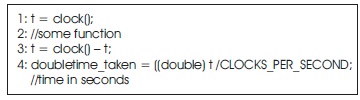
The difference between the two are used to measure the time taken by the function. This difference divided by CLOCKS PER SEC or CPS (the number of clock ticks per seconds) gives the processor time spend for every individual function. Since the insert would not be performed in bulk, the random number produced should be relatively small so as to allow for collisions to deliberately occur.
The CPS of the inserting a record in a program using separate chaining as compared to a program using double hashing helps determine the collision handling scheme. As the number of records inserted increases, it can be intuitively noted that the program will take a longer time to insert. No proportionality relationship can be mapped as insertion depends on the record itself as the ASCII code of the record will be used to generate a key, which is different for various number of records.
The following graph shows the time taken to insert a record after a set of records are already inserted in the hash table. A total of 30 records were inserted for three trails, therefore increasing accuracy and reducing the random error caused by the spread in the id numbers produced by the random function. Figure 1 shows the mean of the three trails taken together.
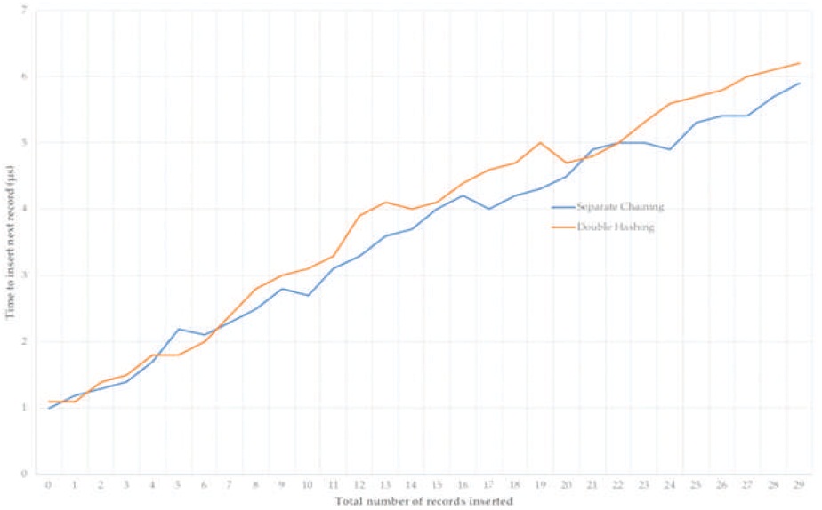
Figure 1. Graph Showing the Relation Between Records Inserted and Time Taken to Insert a Record
There is a positive correlation between the time taken to insert a record and the number of records inserted. Double hashing takes more time to insert records as the table starts filling up. This is because though both hashing functions use the same primary hash function, double hashing requires further computation of a secondary hash function. Hence, it can be concluded that separate chaining works more efficiently for high values of α provided it does not form a linear long chain.
Similarly, this idea could be extended further to increase the number of hashing functions used for a better collision management scheme. However, this would come at the cost of having to calculate mapping keys for collisions.
The basic idea of different accessing methods is to retrieve and update data efficiently. The most appropriate algorithm for hashing in a banking record system to prevent collisions would be separate chaining. Separate chaining shows a slight decline in the time taken to insert a record when inserting over 25 records. However, this comparison is limited by the number of records inserted. Another program could be designed, which reads records from a .csv file and then inserts it into the programs, which hash the records accordingly. Thus, enabling the program to insert a larger number of records at a time without having to individually insert every record.
Physicist Richard Feynman used quantum effects to create new types of computers in 1980s. The concept was using sub-atomic particle behaviour as the stepping stones of computing.
The restrictions of silicon based innovation can be overcome by using quantum PCs (Harrison, 2016). The search performance of a traditional database can be accelerated using a quantum computer. It can also execute a full table scan and find match rows for a complex non-indexed search term. When the traditional disk access is the limiting factor it is likely to be indecisive, an in-memory database quantum database search is a possible improvement.