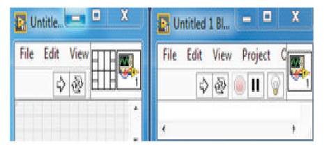
Figure 1. Front Panel and Block Diagram
The main objective of this paper is to simulate scientific calculator using NI LabVIEW software, a graphical programming language to automate the calculation procedure making less paper work for problem solving. In this work, the authors build logics by wiring icons in block diagram which is a graphical source code instead of line of text and the front panel acts as a user interface of the VI to create fully featured scientific calculator. It enables execution highlighting on block diagram and makes the flow of data visible at run-time engine and real-time operating system. This software enables the user to correct the errors with an indication of broken arrow (Run button) on the pull down menu.
A calculator generates step by step procedure for each and every operation. The calculator [9] with scientific features was first identified by Mathatronics Mathatron. It used Reverse Polish notation, LED display and CORDIC algorithm for trigonometric computation [7] in a personal computing device [10]. Later on February 1, 1972, HP-35 [3] the first pocket calculator and the world's first handheld Scientific Calculator was introduced by Hewlett-Packard [4] (HP-9100A). Scientific calculator introduced on January 15, 1974 was one of the most widely used scientific calculators in classrooms [6]. The common brands majorly used were Casio and Sharp. Scientific Calculator [11] generally possess more features than the few basic arithmetic operations of standard calculator [2]. Whenever quick access is needed for any operations (i.e. calculating problems in science, engineering and mathematics); these calculators [8] are widely used. LabVIEW programs are called Virtual Instruments (VIs) [1]. It has three main components – the front panel, block diagram (contains sub VI's, constants, functions i.e. structures, numeric, Boolean, comparison, etc., and wires to build logics), and icon and connector pane. Simulation is carried out based on the logic implemented using functions and icons in block diagram [5]. Educational and Scientific Institutions, Government Organisations are applications of a Scientific Calculator.
After opening software go to File →New VI to create new front panel and the block diagram is shown in Figure 1. Take 1 indicator, 3 controls and enum icon on front panel and take case structure on the block diagram.
Figure 1. Front Panel and Block Diagram
In block diagram, right click →Functions→ Structures palette →Case structure (shown in Figure 2).
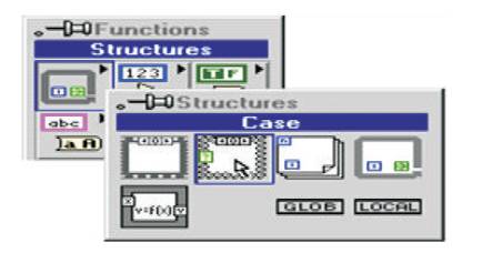
Figure 2. Selection of Case Structure
It consists of 1/more sub diagrams (cases as shown in Figure 3) where only 1 case is visible AND gets executed at a time (all cases are placed one after another). Depending upon the input value given, i.e. (numeric, Boolean AND string controls or enum) to the question mark symbol at the left side of the case structure, it executes one particular sub diagram (case) at that instance [12].
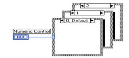
Figure 3. Sub Diagrams in Case Structure
By right clicking on the boundary of the case structure we can find some options as given below in Figure 4.
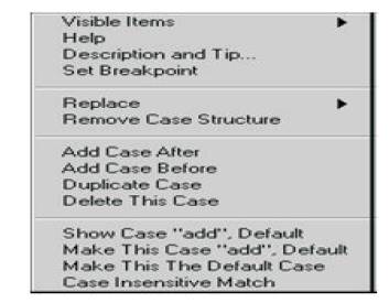
Figure 4. Options in Case Structure
Connect the enum control on block diagram to the case structure to the question mark symbol. After entering all the cases in edit items list, by using 'add case after/before' option we can add the required 25 cases to the case structure and start building logics. Make default case at the top of enum list. Then select required case in the enum icon by giving values in numeric control icons (input 1, input 2, and input 3) and execute the VI (Lab VIEW program) by clicking the run button. Desired result will be displayed in the output icon (numeric indicator). 'N' number of cases can be entered in edit items list on the front panel and added to case as below in Figure 5.
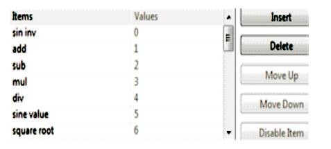
Figure 5. Edit Items Window
The above described procedure is interfaced with NI LabVIEW software and then simulated (run). After simulation, we get the desired outputs in enum.
If any case is not selected on the enum control icon in edit items list, then this case is enabled to perform default operation (sine inverse). To build this logic, connect input 1 to sine inverse icon as shown in Figure 6.
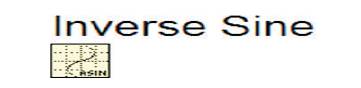
Figure 6. Inverse Sine Icon
The icon's output is given to multiply icon as shown in Figure 7.

Figure 7. Multiply Icon
Another input terminal of this multiplication icon is connected to 180/pi for converting the result from radians to degrees using division icon shown in Figure 8.
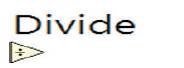
Figure 8. Divide Icon
The output of multiply icon is given to the round to nearest value icon shown in Figure 9 (present in numeric palette).
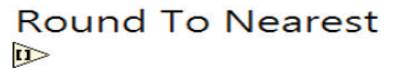
Figure 9. Round to Nearest Icon
In each sub diagram (case), it utilizes inputs based on its logic requirement. In this case we use only input 1 as shown in Figure 11; when inputs 2 and 3 are left free as there is no use of those. If any other case requires 2 or 3 inputs to build logics, then it uses all inputs. When polar case is executed, then theta indicator icon value is displayed. Input 3 is used for x+ fraction case. In enum, select default (sine inverse) case and run the program to execute the above logic and check the result at the indicator icon labelled as output on the front panel as shown in Figure 10.
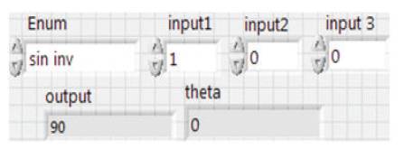
Figure 10. Front Panel of Sine Inverse Case
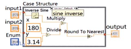
Figure 11. Block Diagram of Sine Inverse Case
The addition case is selected to perform this operation. In this, we use Add icon as shown in Figure 12.
Figure 12. Add Icon
To get the desired result, connect two numeric controls and 1 numeric indicator icons as inputs and output to the add icon, respectively as shown in Figure 14. Addition of two numbers is done by assigning values in numeric controls. In enum select addition case and run the program to execute the above logic and check the output at the indicator icon labelled as output on the front panel as shown in Figure 13.
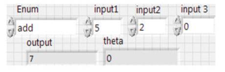
Figure 13. Front Panel of Addition Case
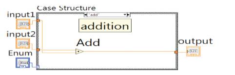
Figure 14. Block Diagram of Addition Case
Subtraction case is selected to perform this operation. Subtract icon is taken as shown in Figure 14.
Then connect two numeric controls and 1 numeric indicator icons as inputs and outputs to the subtract icon as shown in Figure 17. Subtraction of two numbers are done by assigning values in the numeric controls. In enum, select subtraction case and run the program to execute the above logic and check the output at the indicator icon labelled as output on the front panel as shown in Figure 16.

Figure 15. Subtract Icon
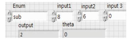
Figure 16. Front Panel of Subtraction Case
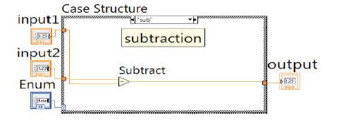
Figure 17. Block Diagram of Subtraction Case
The multiplication case is selected to design this operation. Multiply icon is used to build this logic. To get multiplication of two numbers, connect two numeric controls at the input side of the multiply icon and to view result, connect the output of the multiply icon to the numeric indicator (output icon) as shown in Figure 19. In enum, select multiplication case and run the program to execute the above logic and check the output at the indicator icon labelled as output on the front panel as shown in Figure 18.
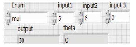
Figure 18. Front Panel of Multiplication Case
The division case is selected to perform this operation. Division icon is used to connect 2 numeric controls as inputs then create 1 numeric indicator icon to view the division of two numbers at the output icon as shown in Figure 21. In enum, select this case and run the program to execute the above logic and check the output at the indicator icon, i.e. output on the front panel as shown in Figure 20.
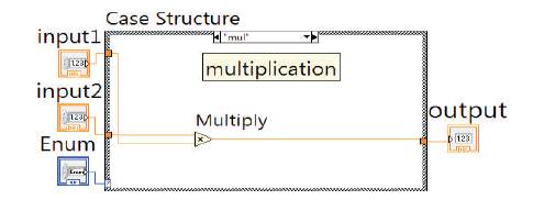
Figure 19. Block Diagram of Multiplication Case
Figure 20. Front Panel of Division Case
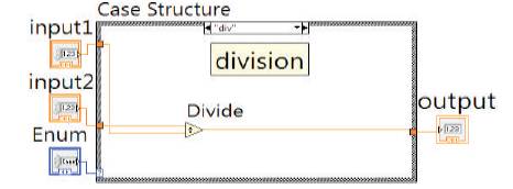
Figure 21. Block Diagram of Division Case
The sine case should be selected to build this logic. We can implement this logic by using a formula node. Block diagram structures the palette formula node and places it inside the case structure, then right click on the formula node add inputs and add outputs to create x and y nodes. X is taken as input where, it is wired to numeric control at the left side and y is taken as output which is connected to the numeric indicator at the right side of the case as shown in Figure 23. Inside the formula node, type the formula using sine command function and end the formula with a semi colon, i.e. sin(x*pi/180); to know the desired result of the sine function pi/180 should be multiplied to the x value to get the result in degrees where the formula, i.e. y=sin(x) gives the sine value in radians. In enum, select sine value case and run the program to execute the above logic and check the output at the indicator icon labelled as output on the front panel as shown in Figure 22.
Figure 22. Front Panel of Sine Value Case
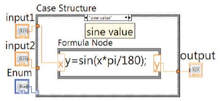
Figure 23. Block Diagram of Sine Value Case
The square root case is selected to perform this logic. In this, we use the formula node by adding input and output as in sin(x) case. Type a formula using square root command function and end it with a semi colon, i.e. y=sqrt(x); as shown in Figure 25. In enum, select this case then run and execute the above logic and check the output at indicator icon labelled as output on the front panel as shown in Figure 24.
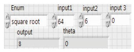
Figure 24. Front Panel of Square Root Case
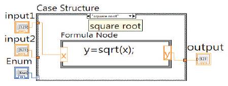
Figure 25. Block Diagram of Square Root Case
The log(x) to base x case is selected to implement this logic. In this, two numeric controls (x & base values) are connected as inputs to the log icon taken from logarithms as shown in Figure 26.
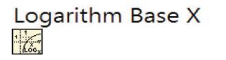
Figure 26. Logarithm Base X Icon
The output terminal of icon is given to output indicator as shown in Figure 28. In enum, select log x to base x case and run the program to execute the above logic and check the output at the indicator icon labelled as output on the front panel as shown in Figure 27.
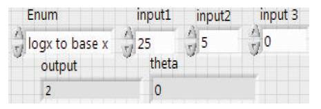
Figure 27. Front Panel of Log x to Base x Case
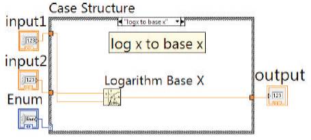
Figure 28. Block Diagram of Log x to Base x Case
The exponential case is selected to design this logic. In this we use exponential icon as shown in Figure 29.
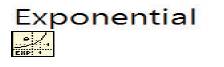
Figure 29. Exponential Icon
1 input and output is given to this icon using numeric control and the indicator as shown in Figure 31. If we want to perform any exponential operation, then go to enum and select this case then run the program to execute the above logic and check the result at the indicator icon labelled as output on the front panel as shown in Figure 30.
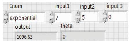
Figure 30. Front Panel of Exponential Case
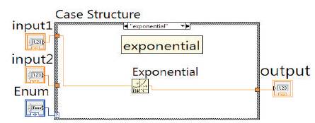
Figure 31. Block Diagram of Exponential Case
The power of 10 case is used to build this logic. In this, we use power of 10 icon as shown in Figure 32.
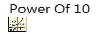
Figure 32. Power of 10 Icon
This has one input and output terminal. Connect the input and output terminals of the above icon to input 1 and output icon as shown in Figure 34. In enum, select power of 10 case and run the program to execute the above logic and check the output at the indicator icon labelled as output on the front panel as shown in Figure 33.
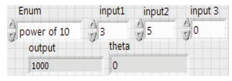
Figure 33. Front Panel of Power of 10 Case
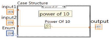
Figure 34. Block Diagram of Power of 10 Case
The yth root of x case is selected to build this logic. In this we use y-th root of x icon as shown in Figure 35.
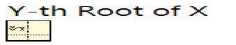
Figure 35. Y-th Root of X Icon
There are two input terminals and 1 output terminal for this icon. Connect the upper (y) and lower (x) input terminals of icon to the 2 numeric controls. Then output of this icon is connected to the numeric indicator as shown in Figure 37. In enum, select yth root of x case and run the program to execute the above logic and check the output at the indicator icon labelled as output on the front panel as shown in Figure 36.
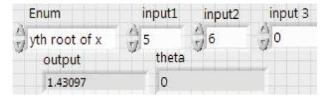
Figure 36. Front Panel of Y-th Root of X Case
The percentage case is selected to build this operation. Division and multiplication icon each are taken to connect two numeric controls to the input terminals of the division icon and output is given as input to the multiplication icon and another input terminal is connected to the numeric constant of value 100. These connections make out a logic to obtain percentage as shown in Figure 39. In enum, select percentage case and run the program to execute the above logic and check the output at the indicator icon labelled as output on the front panel as shown in Figure 38.

Figure 37. Block Diagram of Y-th Root of X Case
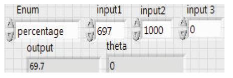
Figure 38. Front Panel of Percentage Case
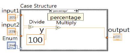
Figure 39. Block Diagram of Percentage Case
The power of x case is used to build this logic. In this, we use power of x icon as shown in Figure 40.
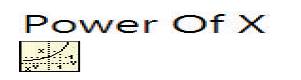
Figure 40. Power of X Icon
Connect 2 numeric controls and 1 numeric indicator to the 2 inputs and 1 output terminals of the icon, respectively. The power of any x value can be obtained by this logic as shown in Figure 42. In enum, select power of x case and run the program to execute the above logic and check the output at the indicator icon labelled as output on the front panel as shown in Figure 41.
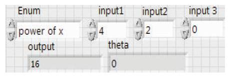
Figure 41. Front Panel of Power of x Case
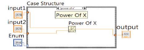
Figure 42. Block Diagram of Power of x Case
The x-inverse case is selected to build this logic. Take a division icon and connect 1 numeric control to the 2nd input terminal of the icon and 1st input terminal is connected to the numeric constant value of 1. Then output of this icon is given to the numeric indicator. By this inverse value of any x number (input 1) is obtained as shown in Figure 44. In enum, select x-inverse case and run the program to execute the above logic and check the output at the indicator icon labelled as output on the front panel as shown in Figure 43.
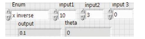
Figure 43. Front Panel of X- Inverse Case
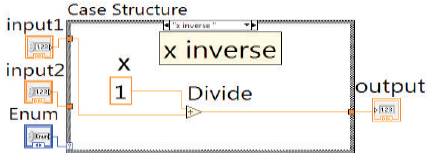
Figure 44. Block Diagram of X- Inverse Case
The x^2 case is taken to build this logic. In this operation, a multiply icon is taken to which only 1 numeric value is connected to the 2 input terminals of the icon and output of this icon is connected to the numeric indicator. In this, the square of any x value is obtained as shown in Figure 46. In enum, select x^2 case and run the program to execute the above logic and check the output at the indicator icon labelled as output on the front panel as shown in Figure 45.
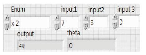
Figure 45. Front Panel of x^2 Case
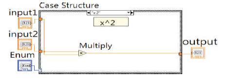
Figure 46. Block Diagram of x^2 Case
The x^3 case is selected to perform this logic. To build this operation, 2 multiply icons are used. Single numeric value is given for 1st multiply icon and the result of this 1st icon with the same numeric value is given as inputs to the 2nd multiply icon then output of this 2nd icon is given to indicator icon to view x^3 value as shown in Figure 48. In enum, select x^3 case and run the program to execute the above logic and check the output at the indicator icon labelled as output on the front panel as shown in Figure 47.
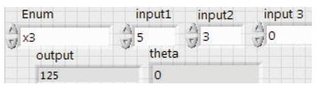
Figure 47. Front Panel of x^3 Case
The cube root of x case is selected to implement this logic. To perform this operation, select y-th root of x icon. But in the place of y, create a numeric constant 3. And the x value of the icon is connected to the numeric control to give input values. Output of this icon is connected to the numeric indicator as shown in Figure 50. In enum, select this case and run the program to execute the above logic and check the output at the indicator icon labelled as output on the front panel as shown in Figure 49.
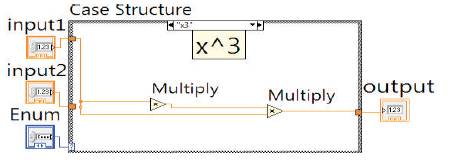
Figure 48. Block Diagram of x^3 Case
Figure 49. Front Panel of Cube Root of x Case
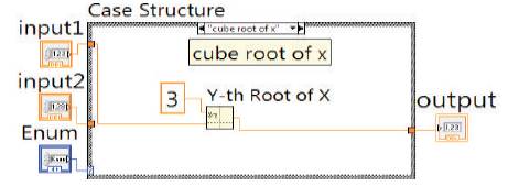
Figure 50. Block Diagram of Cube Root of x Case
The log x case is selected in the case structure to build this logic. To implement this operation, logarithm base 10 icon is taken from logarithms on block diagram. This icon contains 1 input and output terminal each to which 1 numeric control and indicator are connected as shown in Figure 52. In enum, select log x case and run the program to execute the above logic and check the output at the indicator icon labelled as output on the front panel as shown in Figure 51.
Figure 51. Front Panel of Log x Case
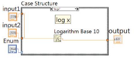
Figure 52. Block Diagram of Log x Case
The log x case is selected to build this logic. In this, we use natural logarithm (ln) icon as shown in Figure 53.
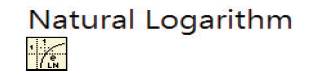
Figure 53. Natural Logarithm Icon
It contains 1 input and output terminal each to which 1 numeric control and indicator is connected as shown in Figure 55. In enum, select ln x case and run the program to execute the above logic and check the output at the indicator icon labelled as output on the front panel as shown in Figure 54.
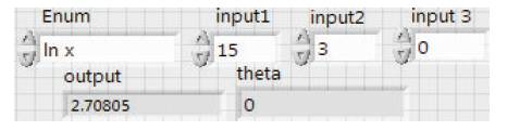
Figure 54. Front Panel of Ln(x) Case
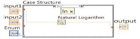
Figure 55. Block Diagram of Ln(x) Case
The cos x case is selected to build this logic. We can implement this logic by using formula node by adding inputs and outputs as in sin(x) case. Inside the formula node, type the formula using cosine command function and end the formula with a semi colon, i.e. y=cos (x*pi/180); to know the desired result of the cosine function pi/180 should be multiplied to the x value to get the result in degrees where the formula y=cos(x) gives the cosine value in radians as shown in Figure 57. In enum, select cosine value case and run the program to execute the above logic and check the output at the indicator icon labelled as output on the front panel as shown in Figure 56.
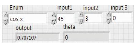
Figure 56. Front Panel of Cos x Case
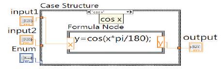
Figure 57. Block Diagram of Cos x Case
The tan x case is selected to build this logic. In this, by using formula node by adding inputs and outputs as in sin(x) case. Inside the formula node, type the formula using tan command function and end it with a semi colon, i.e. y=tan(x*pi/180); to know the desired result of the tan function pi/180 should be multiplied to the x value to get the result in degrees where the formula y=tan(x) gives the sine value in radians as shown in Figure 59. In enum, select tan x case and run the program to execute the above logic and check the output at the indicator icon labelled as output on the front panel as shown in Figure 58.
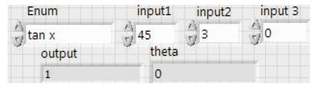
Figure 58. Front Panel of Tan x Case
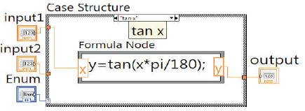
Figure 59. Block Diagram of Tan x Case
The x+ fraction case is selected to build this logic. In this, one divide icon is taken from the block diagram. For this, icon 2 numeric controls are connected as inputs and the output of this icon is connected to the addition icon and another input terminal of addition icon is connected to 3rd numeric control and output of this addition icon is connected to the numeric indicator to obtain the result. In all other cases, we require 1 or 2 inputs, but only in this case we need 3 inputs. So, we should place input 3 icons inside this particular case which is used to connect only in this case as shown in Figure 61. In enum, select x+ fraction case and run the program to execute the above logic and check the output at the indicator icon labelled as output on the front panel as shown in Figure 60.
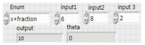
Figure 60. Front Panel of X+ Fraction Case
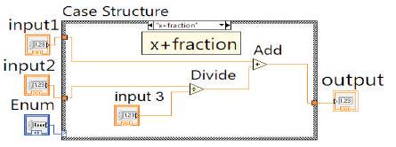
Figure 61. Block Diagram of X+ Fraction Case
The x*10 power of b case is selected to build this logic. In this operation select power of x icon to which input 2 and a constant value of 10 are connected. Output of the above icon and input 1 is connected to multiply icon. Output of this multiply icon is directly given to the indicator icon labelled as output as shown in Figure 63. In enum, select x*10 power of b case and run the program to execute the above logic and check the output at the indicator icon labelled as output on the front panel as shown in Figure 62.
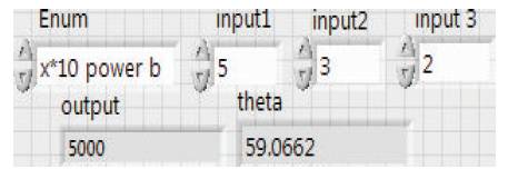
Figure 62. Front Panel of X*10 Power of b Case
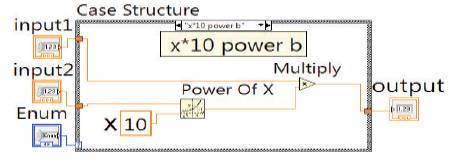
Figure 63. Block Diagram of X*10 Power of b Case
The x-factorial case is selected to implement this logic. Select factorial.vi icon as shown in Figure 64.
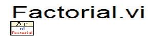
Figure 64. Factorial.vi icon
It consists of only 1 input and output terminal each. Connect a numeric control to the left side of the icon and a numeric indicator at the right side of the icon to obtain the factorial of x values as shown in Figure 66. In enum, select x-factorial case and run the program to execute the above logic and check the output at the indicator icon labelled as output on the front panel as shown in Figure 65.
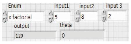
Figure 65. Front Panel of X Factorial Case
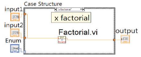
Figure 66. Block Diagram of X Factorial Case
This is selected to perform polar case. We use Real/imaginary to complex icon as shown in Figure 67.

Figure 67. Real/Imaginary to Complex Icon
2 numeric controls (inputs 1 and 2) are connected as inputs for the above icon and output terminal of it is connected as input for complex to polar icon as shown in Figure 68.
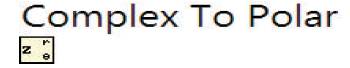
Figure 68. Complex to Polar Icon
The output 1(r) of the above icon is directly connected to the output icon at the right side of the case structure and output 2(e) of the above icon is connected as input to the division icon. Another input terminal of this division icon is connected to the pi value (3.14). A numeric constant (180) and output of divide icon is connected as inputs to the multiply icon. Output of the above icon is connected to numeric indicator to obtain theta value as shown in Figure 70. In enum, select polar form case and run the program to execute the above logic and check the output at the indicator icon labelled as output on the front panel as shown in Figure 69.
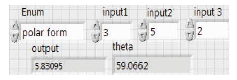
Figure 69. Front Panel of Polar Form Case
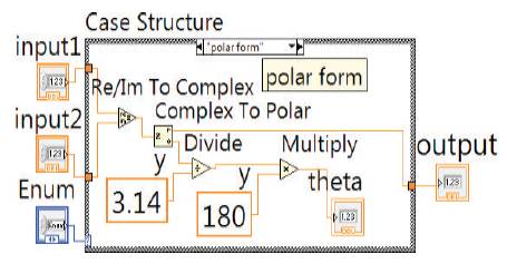
Figure 70. Block Diagram of Polar Form Case
The implementation of scientific calculator using LabVIEW software is simpler and it has many applications. If any terminal of the icon is left free then error occurs as; it contains unwired or bad terminal. Scientific calculators are generally used in higher level math when all the type of mathematical and scientific operations are to be performed. This calculator is usually used by planners, accountants, designers, architects and even professionals in the engineering, mining and mathematical fields for a variety of calculations and by students of science and research and people from a technical background.