The Optimal Power Flow (OPF) is a popularly used method in electrical power system for effective controlled operation and proper planning towards meeting the load growth subjected to meeting various objectives. The chief necessity of the optimization of the power flow is to estimate the proper combination of the controllable parameters like voltage and real power generation at generator buses, tap setting of the transformers in transmission lines and value of compensating capacitors towards minimization of the specific objective functions. A problem with more number of controllable parameters makes the system non-linear and discontinue. So, traditional solution methodologies failed to give an optimized global solution.

The conventional dynamic technique is applied to OPF problem and benders decomposition for effective scheduling in a power system to meet the required demand at minimum production cost [1, 2]. If the price of fuel increases, there will be rise in the generation cost of electric power. This necessitates finding a more feasible way of generating electric power at a minimized cost of the power system while meeting the specific physical and operating constraints.

At power stations, various strategies like installation of electrostatic precipitators and gas scrubbers, replacement of fuel-burners, efficient cleaners and shifting towards low emission fuels are the alternatives for low emission dispatch. These options can be made for long-run planning. In [3], a strategy to minimize emission was proposed.

In power system, minimizing of transmission real power losses can be considered as one of the objective functions for the effective reactive power dispatch. Since minimization of this objective function tends to rise in generator voltages, it results in decrease of the reactive power reserve capacity during contingencies [4]. Minimizing the deviation of load bus voltages from the desired values can be considered as Voltage Stability Index (VSI) objective. Improving the voltage stability margin is also considered as an objective for voltage/reactive power control. Sometimes, this objective minimization gives very different control directions [5].

The literature concentrated on the application of optimization techniques to OPF problems like, linear and non-linear programming [6, 7], Newton's method [8], Quadratic Programming [9], Fast Successive Linear Programming algorithm [10], etc. At present, these evolutionary algorithms are promoted to overcome the drawbacks of the traditional optimization techniques, as their inherent capability is of processing towards the best result and extensive exploration in search space [11] . Minimizing production cost subject to emissions constraints was discussed in [12-14]. The sum of production cost and emission together as an objective function is discussed in [15, 16] . An approach which minimizes the emission and production cost simultaneously was proposed in [17].

The algorithms like Multi-Objective Stochastic Search Techniques (MOSST) [18], Multi-Objective Evolutionary Algorithm (MOEA) [19], Strength Pareto Evolutionary Algorithm (SPEA) [20], Niched Pareto Genetic Algorithms (NPGA) [21] and Non-dominated sorting in Genetic Algorithms (NSGA) [22], etc., can be used to solve multi objective optimization problem. A multi-objective evolutionary algorithm [23] and Goal programming method [24] were applied to environmental/economic power dispatch problem. E-constraint method was proposed to solve multi-objective optimization problems [25–27]. Enhanced Genetic Algorithm based computation technique for multi-objective optimal power flow was proposed in [28]. PSO is used to solve nonlinear optimization problems [29].

The main contribution of this paper is “the application of Nondominated Sorting methodology with Particle Swarm Optimization (NDSPSO)” to find maximum loadability on a given system subjected to satisfy multiple objectives and to find globally compromised solution using fuzzy decision-making tool. The proposed methodology is applied to IEEE-30 bus test system. Some of the results of the proposed method were compared with the results of the existing method [5].

Many of the optimization problems discussed in literature is restricted to either of the certain objectives like Generation Cost, Emission, Loadability, Losses and Voltage Stability Index (VSI) etc. But in practice it is necessary to optimize many of the above objectives simultaneously satisfying equality, inequality and operating constraints. Hence, it is clear that the effectiveness and efficiency of multi-objective algorithm gives best compromised solution subjected to constraints on a system.

A multi-objective optimization technique (NDSPSO) is applied to maximize the system loadability and minimize the other objectives such as Generation Cost, Emission, Losses, and Voltage Stability Index simultaneously by satisfying system constraints.

Aggregating all objectives and constraints, the problem can be formulated mathematically as a constrained nonlinear multi-objective optimization problem as follows:

[1]

Subject to

[2]

[3]

where ‘g’ and ‘h’ are the equality and inequality constraints respectively and ‘x’ is a control vector of dependent variables like slack bus active power generation (p_g,slack ), load bus voltage magnitudes (V_L ) and  generator reactive powers (Q_G ) and vector ‘u’ control  variables like active powers (P_G ) and voltages (V_G ) of generators, transformer tap ratios (T) and shunt compensation (Q_c ). ‘j’ is the total number of objective functions.

The organization of the paper is as follows: Constrained Problem formulation, multi-objective optimization approach with algorithm and corresponding numerical results in sections 1, 2, and 3 respectively.

Multi-objective optimization can have two or more objective functions to be optimized at same time. As a result, there is no unique solution to multi-objective optimization problems, but the aim is to find all possible compromised solutions available in search space (called Pareto front set).

2.1 Generation Fuel Cost

The fuel cost function which satisfies particular operating constraints and practical loading concern can be represented approximately by a simple quadratic function, under the assumption that the incremental cost curves of the generating units are monotonically increasing piecewise linear functions. The fuel cost function of any generator can be mathematically expressed as

[4]

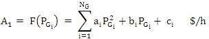
where N_G is the number of generators, a_i , b_i and c_i are the  cost coefficients and p_Gi is the real power output of i^th generator.

2.2 Emission

While minimizing fuel cost of generating units, may produce high levels of SO₂ and NO₂ emissions [30], these  nvironmental concerns are because of using fossil fuels in electric generators, and global warming etc.

Due to the limitations imposed by the Act 1990 [30] , best feasible option is to operate the system as environmental friendly. The total SO_X and Nitrogen oxides NO_X emitted by  E(p ) [5] is

[5]

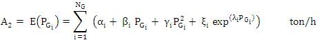
where  α_i, β_i, γ_i, ξ_i and λ_i are emission coefficients of the  i^th  generator.

2.3 Power System Active Power Losses

In power system to enhance power deliver y performance, one of the important issues to be considered is active power loss.

[6]

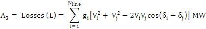
where N_line is total number of transmission lines, g_i is the conductance of i^th line which connects buses i and j. V_i , V_j  and  δ_i, δ_j are voltage magnitude and angle of i^th and j^th buses.

2.4 Voltage Stability Index

L - index (L_j ) [A] of the load buses is considered to monitor j the voltage stability in power system. The value of this L - index is in the range of '0' (no load on the system) to '1' (system voltage collapse). The voltage stability index of j^th bus can be calculated as,

[7]

 

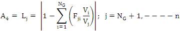
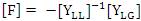
All quantities within the sigma in the RHS of L_j are complex  quantities. The values of [F_ji ] are obtained from Y bus matrix. At all load buses (NL), VSI for the given load condition are computed and the maximum value of L - indices infers the proximity of the system to voltage collapse.

2.5 Loadability

The growth of electricity demands and transactions in power transfer corridors need to increase their loadability. System maximum loadability can be calculated by increasing the system load until the network or equipment constraints, such as thermal, and voltage security limits, are reached [31].

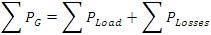
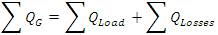
The real and reactive power balance equations at i^th bus can be expressed as

[8]

[9]

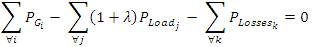
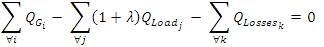
where P_Gi and Q_Gi are the active and reactive power  generations at i^th generator, P_Loadj and Q_Loadj are the real and  eactive power loads at j^th bus under base case condition (λ=0), P_Lossesk and Q_Lossesk are real and reactive power  Losses in k^th transmission line and ‘λ’ is the loadability factor

The system loadability objective can be formulated as:

[10]

Subject to equality and inequality constraints.

3. Constraints

3.1 Equality constraint

This constraint is typically load flow equations.

 

 

3.2 In equality constraints

These constraints represent system operating limits.

3.2.1 Active and reactive power generation constraint

 

 

where P_Gi and Q_Gi are the active and reactive power   generations of i^th  generator P^min_Gi , P^max_Gi , and Q^min_Gi , Q^max_Gi are the corresponding minimum and maximum active and reactive power generation limits of the i^th  generator

3.2.2 Security constraint

 

where S_li is the line MVA flow and S_li^max is the maximum MVA  flow limit of the i^th line, n_l is the total number of lines.

3.2.3 Transformers tap position constraint

 

where T_i^min  and T_i^max are the minimum and maximum tap  positions of the i ^th transformer, respectively, n_t is the total  umber of tap positions.

3.2.4 Bus voltage magnitude constraint

 

where V_i is the i^th bus voltage magnitude, V_i,min and V_i,max are the minimum and maximum voltage magnitude values th of the i^th bus, respectively.

3.2.5 Switchable VAr sources constraint

 

where Q_ci^min and Q_ci^max are the minimum and maximum  values of the reactive power compensated by the i^th  capacitor and n_c is the number of compensators respectively.

A penalty function [32] is added to the objective function, if any of the controllable parameters violates any of the inequality constraints. The methodology of the penalty handling is considered as in [33]. The penalized objective function can be written as the sum of unpenalized objective function (A_m ) plus penalty.

[11]

where R₁ , R₂ , R₃ and R₄ are the penalty quotients having large positive value. The limit values are defined as

[12]

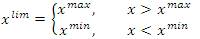
Here ‘x’ is the value of P , V , and Q . g,slack i gi

4. Multi-objective optimization approach

Multi-objective optimization means optimizing multiple objectives of a system simultaneously and systematically. Generally, these objective functions are peculiar and often challenging and inconsistent. Multi-objective optimization with such challenging objectives produces set of optimal solutions, instead of a single optimal solution. The reason for this type of optimality is that, choosing better choice to all objective functions as per the requirement which consist of many issues. These optimal solutions are known as Pareto front sets.

4.1 Non Dominated Sorting

Deb [34] proposed a nondominated sorting method to solve multi-objective optimization problems. There is a requirement to find multiple Pareto front sets in a single run. The fundamental reason behind this multi-objective problem formulation is that it is not probable to have a single solution which optimizes all objectives [35] .

In order to find the superiority of each solution in a population of size ‘N’ with respect to other solutions corresponding to other populations, sorting and comparison operations are performed. This needs C(mN) comparisons for each solution, where m is the number of objectives. At first the nondominated front set is found by using comparison operation on all individuals. In order to find the next front, the comparison procedure for the remaining individuals needs to be repeated.

4.2 Particle Swarm Optimization [36, 43]

Particle swarm optimization conducts its search using a population of particles. Each particle in PSO changes its position according to new velocity and the previous positions in the problem space.

Because of the advantages of the PSO, like simple concept, implementation mechanism, handling of control parameters and finding procedure of the global best solution, it is chosen to implement the defined solution methodology.

In PSO, the particle velocity and the position in (k+1)^th iteration is updated using Eq’s (13) and (14)

[13]

[14]

where k is the iteration count, c₁ and c₂ are acceleration coefficients, rand1 and rand2 are uniformly distributed random numbers in [0 1]. P_best,j is the best position found by the particle j so far, G_best is the position among all particles. Here, the second part is a cognitive part and has its own thinking and memory. The third term is the social parameter on which the particle changes its velocity. ‘w’ is the inertia weight and can be calculated as follows

[15]

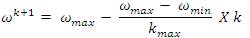
Equations shown in (13) and (14) have three tuning parameters ω, c₁ and c₂ that greatly influence the PSO algorithm performance. The value of ‘ω’ was proposed linearly with time from a value of 1.4–0.5 [36] . As such global search starts with a large weight value and then decreases with time to favor local search over global search [37]. In this paper, the methodology to find values for the tuning parameters and the procedure of updating dynamic inertia weight is implemented [5]. Because this provides a balance between global and local explorations, it needs less number of iterations to get an optimal solution.

4.3 Best compromise solution

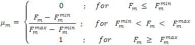
Upon having the multiple nondominated Pareto front sets, fuzzy decision maker is used to select the best compromised solution. The m^th objective function ‘F_m ’ is  represented by a membership function μ_m defined as in  [40]

[16]

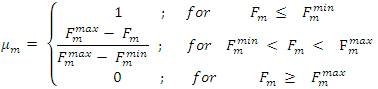
for minimization of objectives and

[17]

 

For each solution in non dominated front set ‘k’, the normalized membership function μ^k is calculated as

[18]

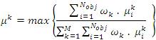
where ‘M’ is the number of non-dominated solutions. The best compromised solution is the one corresponds to the k value of ‘μ^k ’.

5. The computational flow

The main objective is to find the multi-objective optimized loadability estimation on a system by satisfying the constraints. In NR load flow, the reactive generation limits at generator buses are verified and the same bus has been converted into the load bus if any of the minimum/maximum values is violated. The chaotic formula for the inertia weight and the self adaptive method for computing the learning factors beside the proposed algorithm work well for multi-objective optimization problems. The main, noticeable change here is that the increase in the load varies according to remaining objectives to a greater value. So, proper weight should be given to the objectives to get an optimized loadability on a system. As a matter of fact, after acquiring the Pareto front solutions, the decision maker needs to choose one best solution according to the requirement. In this study, W1, W2, W3, W4 and W5 are the weights of corresponding objective functions, respectively, and also

5.1 Implementation of proposed approach

The proposed approach to solve multi-objective problem is described in the following steps:

Step 1: Choose population size ‘M’ and generate the initial population with the control variable bounds, initialize the problem parameters (set iteration count=0).

Step 2: For each of the individual, perform NR load flow and evaluate the objective function values.

Step 3: These solutions constituted as parent solutions.

Step 4: Each solution can be compared with the other solution in the population to find its dominance. Finally, identify different fronts ‘P ’.

Step 5: In order to find the individuals in the next nondominated front, the initial solutions are discounted temporarily and the above procedure is repeated during iteration process. The new solutions are called as offspring solutions.

Step 6: Perform non-dominated sorting on the combined solutions (parent+off-spring) and identify different fronts ‘P ’.

Step 7: Crowding distance operation is performed on the entire set of solutions. This operation requires sorting the population according to each objective function value in ascending order of magnitude.

Step 8: The boundary values are assigned to an infinite distance value for each of the objective function. For the remaining population a distance value equal to the absolute normalized difference in the function values of two adjacent populations is assigned.

Step 9: This calculation is performed for all objectives.

Step 10: The sorting is performed on a given solutions according to their crowding distances and increases the iteration count.

Step 11: Step 5 to Step 10 are repeated till maximum iterations reached

Step 12: Then the member ship values for non-dominated solutions in the Pareto-front are calculated. The final solution is chosen based on the operator's requirements.

6. Numerical results

In this study, the standard IEEE 30-bus, 6-unit test system is considered to investigate the effectiveness of the proposed approach. The system data is taken from [41, 42].

The entire analysis is divided into cases I, II, III, IV and V, which corresponds to single, two, three, four and five objectives optimization problem respectively. The detailed analysis of each case is presented in the following sections. Some of the results of the proposed method are compared with the existing method [5] and are given in Appendix.

6.1 Case – I (Single objective)

The result of control variable variation corresponding to the multiple objectives is given in Table 1. It is observed that the minimization of cost function results in increase of the emission by a factor of 0.7904, losses by 1.9874 and VSI by 0.0448 (all factors are with respect to their minimized values). Table 1 reveals that the minimization of emission function results in increase of the cost by a factor of 0.1801, losses by 0.0709, and VSI by 0.0185. Minimization of losses in the system increases the cost by a factor of 0.2089, emission by 0.0119, and VSI by 0.1574. Similarly minimization of VSI results in increase of the cost by a factor of 0.01663, emission by 0.5745, and losses by 2.2839. In all the above cases there is no chance for getting loadability. But, from the last column of the Table.1, maximization of the loadability on a system results in increase of the cost by a factor of 0.7357, emission by 10.043, losses by 4.2387 and VSI by 0.59103. It is observed that maximizing loadability increases other objectives.

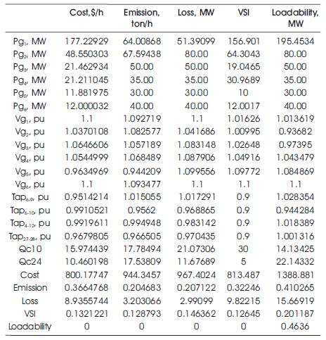
Table 1. Control variables related to multiple objectives

6.2 Case – II (Two objectives)

In this case, the proposed methodology handles two objectives together as multi-objective optimization problem. For each combination there are nine sets, which are selected based on the distribution of weights between objectives. The results of the best compromised over Pareto optimal solutions for Cost-Emission combination is given in Table 2.

Table 2. Multi-objective optimized result for different sets (weight factors)

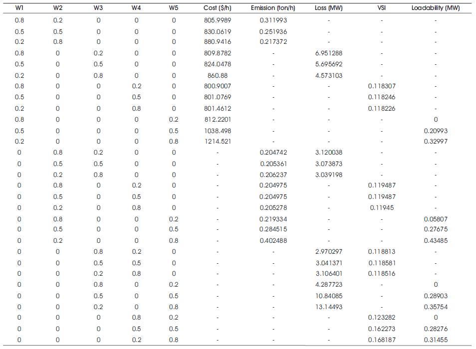
Table 3. Multi-objective result for different weight factors (Two objectives)

Selective analysis is given for the remaining combinations Table 3.

Table 3 reveals that the estimation of loadability has great impact on emission. Because, for Emission-Loadability combination and of 0.8-0.2 set has a very less possibility of increase in loadability by a factor of 0.05807, and for the other combinations, the loadability factor is zero. Highest loadability factor (0.43485) is possible with the maximum emission (0.402488 ton/h). Due to space limitation, two dimensional plots for the following combinations are shown in Figure 1.

 

 

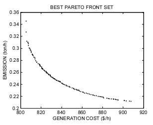
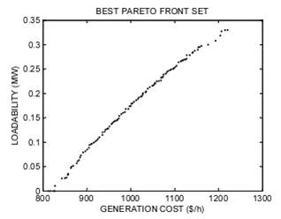
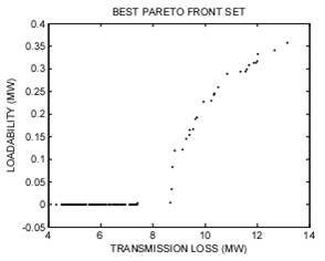
Figure 1. Two dimensional best Pareto-optimal fronts (a) Cost – Emission (b) Cost – Loadability (c) Loss – Loadability

6.3 Case – III (Three objectives)

Here in this case three objectives are considered to form multi-objective optimization problem. With three objectives, ten combinations are possible. For each combination, the possible number of sets is 34 based on weights distribution, here some sample sets are considered for each combination and are tabulated in Table 4, which shows the effectiveness of the algorithm.

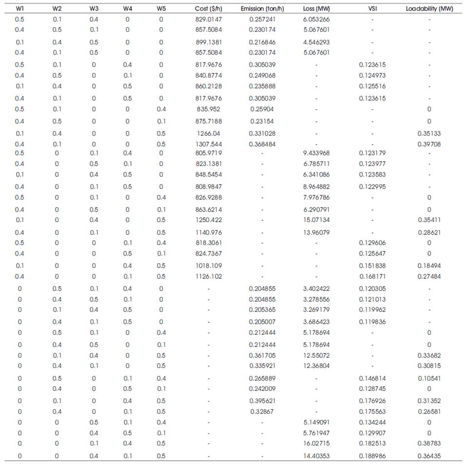
Table 4. Multi-objective result for different weight factors (Three objectives)

From Table 4 it is clear that, the loadability factor can be increased based on the emission objective, as in the previous section, the maximum loadability factor can be obtained with the emission objective. In that case, the cost, losses and VSI are increased drastically to higher values. The generated Pareto fronts confines to entire trade-off regions; this is because of the effectiveness of the proposed methodology. The three dimensional Pareto fronts for different objective function is shown in Figure 2.

 

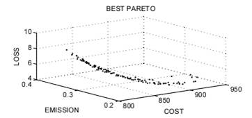
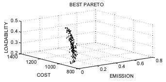
Figure 2. Three dimensional Pareto fronts for different objective functions (a) Cost-Emission-Loss (b) Cost-Emission- Loadability

6.4 Case – IV (Four objectives)

To show the effective results, four objective functions together are formulated as a multi-objective optimization problem. There are five possible combinations with five objectives. For each combination, there are 84 possible sets. Three dimensional Pareto fronts are shown in Figure 3 and the corresponding multi-objective obtained results are tabulated in Table 5.

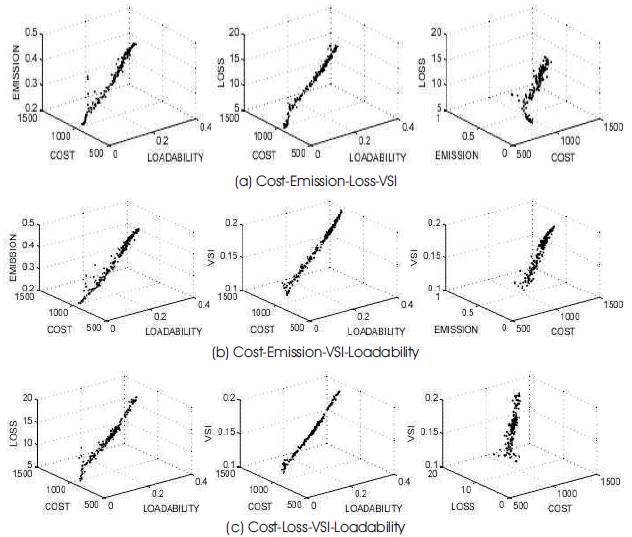
Figure 3. Three dimensional Pareto fronts for different objective functions with one objective constant at one time

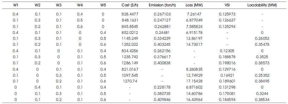
Table 5. Multi-objective result for different weight factors (Four objectives)

It is very interesting point to note from the Table 5 is that, if the equal weight (0.4-0.4) is given for the loadability with the cost and emission objectives resulting in zero loadability. Less loadability is possible with the 0.5 weight for loadability. The emission objective plays a major role to decide the loadability on a system.

6.5 Case – V (Five objectives)

This is very critical section as it combines all the considered five objectives combined together to form the complete analytical effectiveness of the proposed algorithm. This section validates the proposed hypothesis. There are 126 possible sets with these five objectives. The corresponding values for some of the sets with different weights distribution is given in Table 6.

The possible minimum loadability factor is 0.02824 on a system and the maximum loadability is 0.37067. The minimum cost obtained may be around 830 $/h, minimum emission may be around 0.210 ton/h, minimum losses may be around 5.14 MW, and the minimum VSI may be around 0.131. If the loadability increases, the cost, emission, loss and VSI are increased to its maximum values.

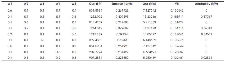
Table 6. Multi-objective result for different weight factors (Five objectives)

Conclusion

The stated hypothesis has been proved and validated with proposed NDSPSO algorithm. The handling of the multiple objectives needs a lot of expertise and estimating simultaneous control actions towards the objective optimization has been validated with the proposed method. The objectives generation cost, emission, loss, VSI and loadability are optimized subjected to equality, inequality and physical constraints. The loadability on a given system is possible by the variation of the other objectives which reduces the network expansion cost for a short term planning. The proposed evolutionary algorithm named “NDSPSO” shows its capability to handle different objectives based on its nature (i.e minimizing certain objectives and simultaneously maximizing certain objectives). The fuzzy decision making tool to select best Pareto front from the generated Pareto optimal solutions proves its effectiveness in selection of globally best solution. The developed code takes around 60-80 seconds for the combinations without loadability objective and with the loadability objective; it takes around 400-450 second because of the loadability calculation (up to five digits) in step wise. Since the proposed methodology uses the calculation of acceleration coefficients and inertia weight based on the nature of the solution and it can be applied to any type of the objectives

Appendix

The results validation of proposed method is compared with the existing method [5] and is tabulated in Table 7. From Table 7, it is observed that, the proposed methodology yields better results.

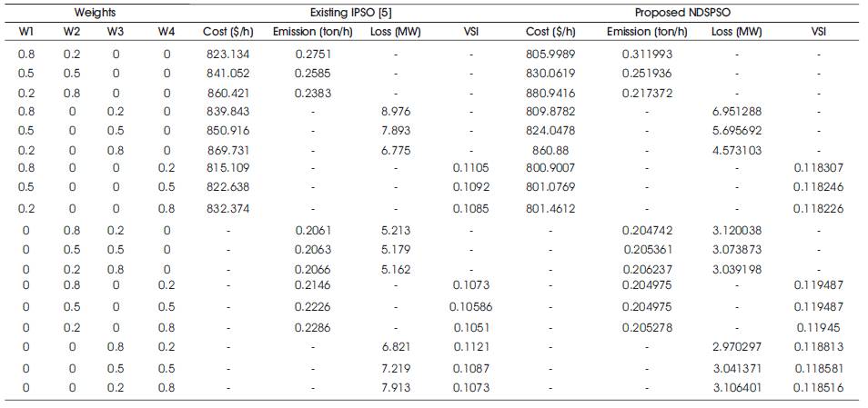
Table 7. Comparison between Multi-objective results for IPSO & NDSPSO

References

[1]. Costa. A.L, Simoes Costa. A., (2007). “Energy and ancillary service dispatch through dynamic optimal power flow,” Electrical Power Systems Research, Vol.77, No.8, pp. 1047-1055.

[2]. Martinez-Crespo. J, Usaola. J, Fernandez. J.L, (2007). “Optimal security constrained power scheduling by Benders decomposition,” Electrical Power Systems Research, Vol.77 No. 7, pp. 739-753.

[3]. A. A. El-Keib, H. Ding, C.C. Carroll, etal., (1991). “Current Challenges for the Electric Power Industry,” U.S. Dept of Energy., Workshop of Real Time Control and Operation of Electric Power Systems, Denver, Colorado, Nov.

[4]. Bansilal, Thukaram. D, Parthasarathy., (1996). “Optimal reactive power dispatch algorithm for voltage stability improvement,” Electric Power Energy Systems, Vol. 18, No.7, pp. 461-468.

[5]. T.Niknam, M.R.Narimani, J.Aghaei, R.Azizipanah- Abarghooee., (2012). “Improved particle swarm optimization for multi-objective optimal power flow considering the cost, loss, emission and voltage stability index,” IET Generation, Transmission & Distribution., Vol. 6, No. 6, pp. 515-527.

[6]. Momoh, JA., El-Hawary, ME., Adapa R., (1999). “A review of selected optimal power literature to 1993. Part I: non-liear and quadratic programming approaches,” IEEE Transactions on Power Systems., Vol. 14, No. 1, pp. 96- 104.

[7]. Momoh, JA., El-Hawary, ME., Adapa R., (1999). “A review of selected optimal power literature to 1993. Part II:Newton, linear programming and interior point methods,” IEEE Transactions on Power Systems., Vol. 14, No. 1, pp. 105-111.

[8]. H. Ambriz-Perez., E. Acha., C.R. Fuerte-Esquivel., De La Torre A., (1998). “Incorporation of a UPFC model in an optimal power flow using Newton's method,” IEEE Proceedings on Generation Transmission Distribution., Vol. 145, No. 3, pp. 336-344.

[9]. C.R. Fuerte-Esquivel., E. Acha., H. Ambriz-Perez, (2000). “A Comprehensive Newton-Raphson UPFC Model for the Quadratic Power Flow Solution of Practical Power Networks,” IEEE Transactions on Power Systems., Vol. 15, No. 1, Feb, pp. 102-109.

[10]. Khaled Z., Sayah S., (2008). “Optimal power flow with environmental constraints using a fast successive linear programming algorithm, applications to the Algerian power system,” Energy Conversion and Management., Vol. 49, No. 11, pp. 3363-3366.

[11]. Taher Niknam., Mohammad rasoul Narimani., Masoud Jabbari., Ahmad Reza Malekpour, (2011). “A modified shuffle frog leaping algorithm for multi-objective optimal power flow,” Journal of Energy., Vol. 36, pp. 6420- 6432.

[12]. S.F. Brodsky and R.W. Hahn., (1986). “Assessing the influence of power pools on emission constrained economic dispatch,” IEEE Transactions on Power Systems., Vol. PWRS-1., Feb.

[13]. J.B. Cadogan and L. Eisenberg., (1981). “Sulfur- Oxide emissions management for electric power systems,” IEEE Transactions on Power App. and Systems., Vol PAS-96, March.

[14]. O.E. Finningan and A.A. Fouad., (1974). “Economic Dispatch with Pollution Constraints,” Paper C 74 1555-8, IEEE PES Winter Meeting, New York, NY, Jan.

[15]. J.K. Delson, (1974). “Controlled emission dispatch,” IEEE PES Winter meering.

[16]. J.S. Helsin and B.F. Hobbs., (1989). “A multiobjective production costing models for analysing emission dispatching and fuel switch,” IEEE Transactions on Power Systems, Vol. 4, No. 3., Aug.

[17]. T.A. Ferrar, (1974). “Effluent charges – A price on pollution,” Atmospheric Environment, Vol. 8.

[18]. Coello CAC., (1999). “A comprehensive survey of evolutionar y-based multi-objective optimization techniques,” Knowledge Information System., Vol. 1, No. 3, pp.269-308.

[19]. Toffolo A, Lazzaretto A., (2002). “Evolutionary algorithms for multi-objective energetic and economic optimization in thermal system design,” Energy., Vol. 27, No. 6, pp. 549-567.

[20]. Abido MA., (2003). “Environmental /economic power dispatch using multi-objective evolutionary algorithms,” IEEE Transactions on Power Systems., Vol. 18, No. 4, pp.1529-1537.

[21]. Andrew K., Haiyang Z., (2010). “Optimization of wind turbine energy and power factor with an evolutionary computation algorithm,” Energy., Vol. 35, No. 3, pp. 1324- 1332.

[22]. N Srinivas and Kalyanmoy Deb., (1994). “Multiobjective Optimization Using Nondominated Sorting in Genetic Algorithms,” Evolutionary Computation., Vol. 2, No. 3, pp. 221-248.

[23]. M.A. Abido., (2003). “A novel multiobjective evolutionary algorithm for environmental/economic power dispatch,” Electric Power Systems Research., Vol 65, pp. 71-81.

[24]. B.S. Kermanshahi, Y. Wu, K. Yasuda, R. Yokoyama., (1990). “Environmental marginal cost evaluation by noninferiority surface,” IEEE Transactions on power systems., Vol 5, No. 4., pp. 1151-1159.

[25]. R. Yokoyama, S.H. Bae, T. Morita, H. Sasaki., (1988). “Multi objective generation dispatch based on probability security criteria,” IEEE Transactions on power systems, Vol. 3, No. 1., pp. 317-324.

[26]. A.A. Abou El-Ela, M.A. Abido., (1992). “Optimal operation strategy for reactive power control in: Modelling, Simulation and Control, part A,” Vol. 41., AMSE Press., pp. 19-40.

[27]. Y.T. Hsiao, H.D. Chiang, C.C. Liu, Y.L. Chen., (1994). “A computer package for optimal multi objective VAR planning in large scale power systems,” IEEE Transactions on Power Systems, Vol. 9, No. 2., pp. 668-676.

[28]. M. Sailaja Kumari, Sydulu Maheswarapu., (2010). “Enhanced Genetic Algorithm based computation technique for multi-objective optimal power flow solution,” Electrical Power and Energy Systems., Vol. 32., pp. 736-742.

[29]. Kennedy J, Eberhart R., (1995). “Particle Swarm Optimization,” IEEE International conference on Neural Networks, Vol. 4., pp. 1942-1948.

[30]. El-Keib. A. A, Ma. H, Hart. J. L., (1994). “Economic Dispatch in view of the clean AIR ACT of 1990,” IEEE Transactions on Power Systems, Vol. 9, No. 2., pp. 972-978.

[31]. Ya-Chin Chang, Rung-Fang Chang, Tsun-Yu Hsiao, and Chan-Nan Lu., (2011). “Transmission System Loadability Enhancement Study by Ordinal Optimization Method”, IEEE Transactions on power systems, Vol. 26, No. 1., pp. 451-459.

[32]. Lai. LL, Ma JT, etal., (1997). “Improved genetic algorithms for optimal power flow under both normal and contingent operation states,” Electric Power Energy Systems., Vol. 19, No. 5., pp. 287-292.

[33]. Alsac O, Scott B., (1974). “Optimal power flow with steady state security,” IEEE Transactions on Power Apparatus Systems., Vol. 93, No. 3.

[34]. Kalyanmoy Deb, Samir Agarwal, Amrit Pratap, and T Meyarivan., “A Fast Elitist Non-Dominated Sorting Genetic Algorithm for Multi-Objective Optimization: NSGA-II,” Kanpur Genetic Algorithms Laboratory, IIT Kanpur, http://www.iitk.ac.in/kangal.

[35]. Srinivas. N, Deb. K., (1995). “Multi- Objective function optimization using non-dominated sorting genetic algorithms,” Evolutionary Computation, Vol.2, No. 3, pp. 221-248.

[36]. Shi. Y, Eberhart. R., (1998). “A modified particle swarm optimizer,” Proceedings of the IEEE international conference on evolutionary computation., Piscataway, NJ: IEEE Press., pp. 69-73.

[37]. Eberhart. R, Shi. Y., (1998). “Computation between genetic algorithms and particle swarm optimization,” Proceedings of the 7th annual conference on evolutionary programming., Berlin: Springer; pp. 611- 618.

[38]. Caponetto. R, Fortuna. L, Fazzino. S, Xibilia. M.G., (2003). “Chaotic sequences to improve the performance of evolutionary algorithms,” IEEE Trans. Evol. Comput., Vol. 7, No. 3, pp. 289-304.

[39]. Jong-Bae Park, Yun-Won Jeong, Hyun-Houng Kim and Joong-Rin Shin., (2006). “An Improved Particle Swarm Optimization for Economic Dispatch with Valve-Point Effect,” International Journal of Innovations in Energy Systems and Power., Vol. 1, No. 1., pp. 1-7.

[40]. J.S. Dhillon, S.C. Parti, D.P. Kothari, (1993). “Stochastic economic emission load dispatch,” Electric Power Syst. Res., Vol. 26., pp. 179-186.

[41]. O. Alsac, B. Stott., (1973). “Optimal Load Flow with steady state security,” IEEE PES summer meeting & EHV/UHV conference., July, pp. 745-751.

[42]. M.A. Abido., (2002). “Optimal power flow using Tabu Search Algorithm,” Electric Power Components and Systems, Vol. 30., pp. 469-483.

[43]. M.A. Abido., (2002). “Optimal power flow using particle swarm optimization,” Electric Power and Energy Systems, Vol. 24., pp. 563-571.