It is known that analyzing the systems with respect to probability of success or failure is a combinatorial problem. Since the value of the probability of an event lies between zero and one, certain combinations will be reduced if a reasonably accurate assessment can be made which shall be based on some approximations.

Further, so far the probabilistic expressions or indices based on the probabilities of components and events have been discussed.

In general, the probabilistic indices are classified as:

• Basic probability indices
• Performance indices

The basic probability indices of systems can be obtained with approximate evaluations of reasonably accurate predictive assessment and it will be discussed in the paper. The performance indices are engineering system oriented and they can be defined according to the specific system subsystem under consideration. It is well known that component redundancy will be leading to better reliability as compared to that of unit redundancy configurations for time independent probabilities. Power system reliability indices such as multi-state stationary availability, the expected unsupplied demand, the loss of load probability and total failed system probability are determined using the technique of Ushakov [2].

A methodology for reliability evaluation and optimization of non-repairable dissimilar component consisting of series parallel configuration for cold-standby redundant system using shortest path technique is proposed [3]. Limit reliability functions are applied to find the reliability of twostate large non-repaired systems composed of independent components [4,5]. Reliability function and the mean time to failure are used to derive hot and cold reliability equivalence factors [6] of a parallel- series system. It is assumed that the system components are independent and identical.

In this paper, exponentially distributed failure rate of the components will be considered for unit or component redundancies. Further, basic probability indices are defined in the literature [8-10]. However, it appears that no attempt has been made to analyze systems with various configurations. In this paper, the basic probability indices that will be defined are equivalent failure rate, mean or average outage time and average annual outage time. In this paper, evaluation of performance indices for various system configurations like series, parallel, seriesparallel, parallel-series configurations and complex systems have been dealt with deriving generalized expressions for 'n' component repairable systems and applied to Power System network [1] using Cutsets.

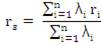
It is well known that the basic probability indices r_s , λ_s, U_s are already defined for approximate system reliability analysis [8] and they are expressed as:

[1]

[2]

[3]

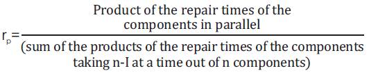
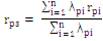
It is well known that the basic probability indices r_p , λ_p , U_p are already defined for approximate systems reliability analysis [8] for two (or) three components in parallel only. In this section, generalized expressions will be derived for ncomponents in parallel. Now the equivalent repair rate of the system can be expressed as:

 

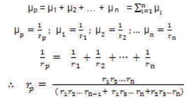
The denominator is referred to as sum of the products form.

 

[4]

and in order to find equivalent failure rate, consider the unavailability of the system as:

[5]

 

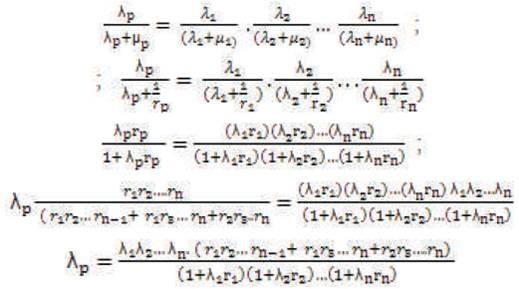
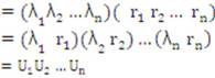
Now, neglecting the terms

 

[6]

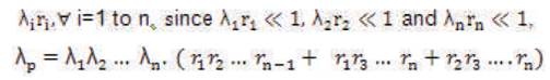
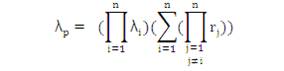
and

[7]

It appears in the literature that no attempt has been made to derive generalized expressions of 'm' series configurations connected in parallel and 'n' configurations are connected in each series configurations as shown in Figure 1(a) and corresponding simplifications are shown in Figure 1 (b) and ( c).

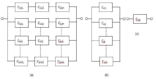
Figure 1. Generalized configuration of unit redundancy in (a) and corresponding simplifications in (b) and ( c)

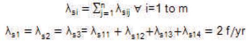
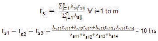
Let λsij be the failure rate of j^th component in the I^th series configuration, i.e., Csij, ∀ i=1 to m; j=1 to n,

rsij be the repair time of j^th component in the I^th series configuration of the component Csij,

∀ i=1 to m; j=1 to n respectively.

Let λ_si , be the Equivalent failure rate of i^th series configuration C_si , ∀ i=1 to m.

r_si, be the Mean outage time of i^th series configuration C_si , ∀ i=1 to m.

U_si, be the Average annual outage time of i^th series configuration C_si , ∀ i=1 to m.

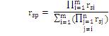
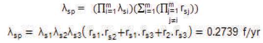
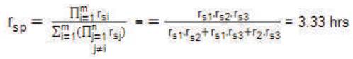
Let λsp be the equivalent failure rate of the system; rsp be the Mean outage time of the system.

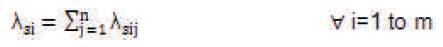
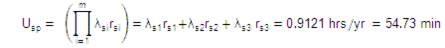
Usp be the Average Annual outage time of the system. Thus, λsi can be obtained as:

[8]

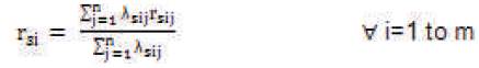
and rsi can be obtained as:

[9]

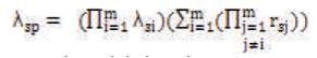
Therefore, λ_sp can be obtained as:

[10]

and hence rsp can be obtained as:

[11]

and Usp can be obtained using

[12]

The generalized configuration of 'n' parallel configurations connected in series and 'm' components are connected in each parallel configuration as shown in Figure 2 (a) and the corresponding simplifications in Figure 2 (b) and ( c). respectively.

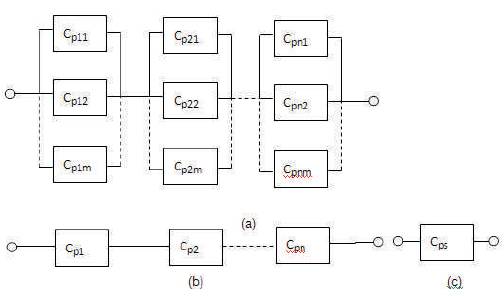
Figure 2. Generalized configuration of component redundancy in (a) and corresponding simplifications in (b) and (c)

Let Cpij be the j^th component in I^th parallel configuration ∀ i=1 to n; j=1 to m respectively

Cpi be the single equivalent configuration of the I^th Parallel configuration, i=1 to n

Let λpij be the failure rate of j^th component C_pij in I^th Parallel configuration, ∀ i=1 to n; j=1 to m respectively.

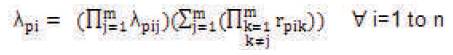
r_pi be the repair time of the j^th component C_pij in I^th Parallel configuration, ∀ i=1 to n respectively.

Let λ_pi be the equivalent failure rate of I^th parallel configuration, C_pi , ∀ i=1 to n

rpi be the Mean outage time of i^th parallel configuration, C_pi , ∀ i=1 to n.

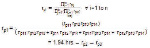
λ_ps , r_ps , U_ps have been already defined in 1.1(Configuration) Now expressions for r_ps , ∀ i=1 to n can be obtained as :

[13]

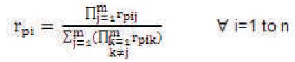
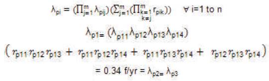
Now λ_pi , ∀ i=1 to n can be obtained as:

[14]

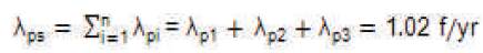
Now λ_ps can be obtained as:

[15]

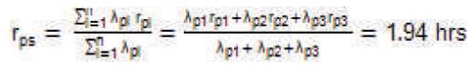
Now r_ps can be obtained as:

[16]

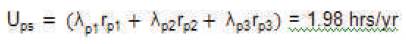
and hence, U_ps can be obtained as:

[17]

2.1.1 Unit redundancy configuration

Consider the unit redundancy configuration shown in Figure 1 (a), it is assumed that the component failures are exponentially distributed with constant hazard rate function (λ).

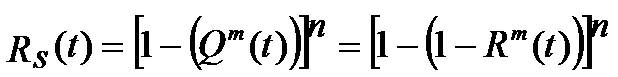
The generalized expression for reliability of the unit redundancy configuration with time independent probabilities is given by:

[18]

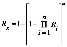
where R_i is probability of success of i^th component

Similarly, the generalized expression for reliability of the unit redundancy configuration with time dependent probabilities can be expressed as:

[19]

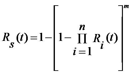
where R_i (t) is the survivor function of i^th component

2.1.2 Component redundancy configuration

Consider the component redundancy configuration shown in Figure 2 (a). It is assumed that the component failures are exponentially distributed with constant hazard rate function (λ).

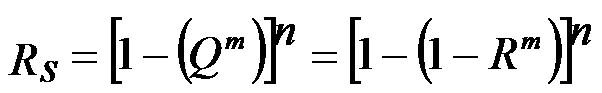
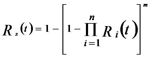
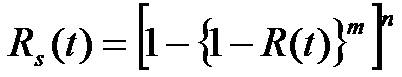
The generalized expression for reliability of the component redundancy configuration with time independent probabilities is given by:

[20]

Therefore, the generalized expression for reliability of the component redundancy configuration with time dependent probabilities can be expressed as:

[21]

Consider the configurations of unit and component redundancies as shown in Figure 1 (a) and Figure 2 (a) respectively. Assuming that each component has a failure rate of 0.1 failures/year, the probability of system surviving after one year can be determined as follows:

Here λ₁=λ₂=0.1 failures/year

• Case 1: Unit redundancy

 

Let n=2, m=2

[22]

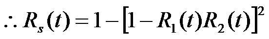
and R₁ (t)=R₂ (t)=e^-λt

[23]

• Case 2: Component redundancy:

 

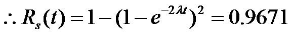
Here n = 2, m=2, R(t)= e^-λt

[24]

Therefore, “component redundancy is better than unit redundancy for exponential distribution also”. However, as already been derived, basic probability indices can also be evaluated using approximate system reliability analysis.

2.2.1 Series and Parallel Configurations

Consider that four components in a system each having failure rates of 0.2 f/yr and repair time of 4 hrs respectively. The basic probability indices for series and parallel systems for the system having two, three, four components respectively can be obtained as follows:

Here n = 4; λ₁ = λ₂ = λ₃ = λ₄ = 0.2 f/yr; r₁ = r₂ = r₃ = r₄ = 4 hrs;

Series system

• 2 components in series

The equivalent failure rate of system is λ_s = λ₁ + λ₂ = 0.4 f/yr

The mean outage time of the system r_s is:

 

• 3 components in series

 

• 4 components in series

 

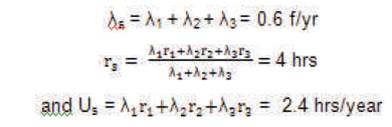
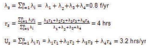
Thus, it can be observed that, in a series system, for the same failure rate and repair time of the components:

• The equivalent failure rate of the system will increase as the number of components increase
• Mean repair time is constant
• The average annual outage time increases as the number of components increase.

Parallel system

• 2 components in parallel:

 

• 3 components in parallel:

 

• 4 components in parallel:

 

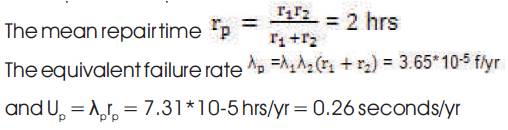
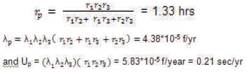
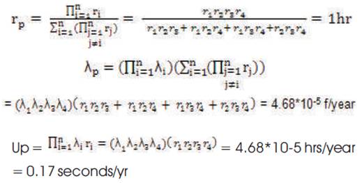
Thus, it can be observed that, in a parallel system, for the same failure rate and repair time of the components:

• The equivalent failure rate of the system increases as the number of components increase
• The Equivalent repair time (Mean outage time) decreases as the number of components increase
• The average annual outage time decreases as the number of components increase.

Therefore, it can be observed that for the same number of components and the same failure and repair data of the components, series system has more equivalent failure rate than that of the parallel system. Also, the mean outage time and average annual outage time is more for series system than that of the parallel system, i.e. in parallel systems, the unavailability is much less than that of the series system.

2.2.2 Series - Parallel and Parallel – Series Configurations

Consider that there are four components in series configuration, having failure rates of 0.2, 0.4, 0.6, 0.8 f/yr and repair times of 20, 15, 10 and 5 hrs respectively and in parallel configuration having three such series configurations having the same failure rates and repair times of components. To find the basic probability indices of Series-Parallel configuration for the Figure in 2 (a).

r_s11 = 20 hrs;  r_s12 = 15 hrs;  r_s13 = 10 hrs;  r_s14 = 5 hrs;
λ_s21 = λ_s31 = λ_s11 = 0.2 f/yr;  λ_s22 = λ_s32 = λ_s12 =0.4 f/yr;
λ_s23 = λ_s33 = λ_s13 = 0.6 f/yr;  λs24 = λ_s34 = λ_s14 = 0.8 f/yr;

The equivalent failure rate of series configurations will be equal to:

 

and the mean outage time of the series configuration is:

 

The equivalent failure rate of the system having seriesparallel configuration is

 

The mean outage time of the system having seriesparallel configuration is:

 

Therefore, the average annual outage time of the system having series-parallel configuration is:

 

Consider that there are four components in parallel configuration, having failure rates of 0.2, 0.4, 0.6, 0.8 f/yr and repair times of 20, 15, 10 and 5 hrs respectively and having three such parallel configurations to be connected in series having same failure rates and repair times of components. The basic probability indices of Parallel-series configuration can be obtained as follows:

Here n=3; m=4; λ_p11 = 0.2 f/yr;  λ_p12 = 0.4 f/yr;  λ_p13 = 0.6 f/yr;  λ_p14 = 0.8 f/yr

r_p 11 = 20 hrs; r_p 12 = 15 hrs; r_p 13 = 10 hrs; r_p 14 = 5 hrs;
λ_p 21 = λp 31 = λ_p 11 =0.2 f/yr; r_p 21 = r_p 31 = r_p 11 = 20 hr;
λ_p 22 = λp 32 = λ_p 12 =0.4 f/yr; r_p 22 = r_p 32 = r_p 12 = 15 hr;
λ_p 23 = λp 33 = λ_p 13 = 0.6 f/yr r_p 23 = r_p 33 = r_p 13 = 10 hr;
λ_p 24 = λp 34 = λ_p 14 = 0.8 f/yr r_p 24 = r_p 34 = r_p 14 = 5 hr;

Now, the equivalent failure rate of the parallel configurations will be equal to:

 

The mean outage time of the parallel configurations is:

 

Therefore, the equivalent failure rate of the system is:

 

The mean outage time of the system is:

 

and the average annual outage time will be

 

Therefore, for the same number of components, failure rates and repair times of the system, it has been observed from examples that,

• The equivalent failure rate increases from series-parallel-series configuration
• Mean outage time decreases from series-parallel to parallel-series configuration.
• The Average annual outage time increases from series-parallel to parallel-series configuration.

The above observations are based on unequal failure rates/ repair times of the components.

2.2.3 Unit and component redundancy

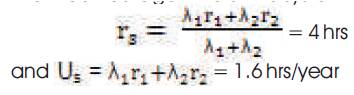
Consider that there are two components in a series configuration each having failure rates of 0.2 f/yr and repair times of 20 hrs respectively and having such two series configurations to be connected in parallel having same failure rates and repair times of components. The basic probability indices of series-parallel system can be obtained as follows:

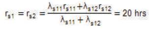
Here n=2;  m=2;  λ_s11 = λ_s12 = 0.2;  r_s11 = r_s12 = 20 hrs

The equivalent failure rate of series configurations will be equal to:

 

and the mean outage time of the series configuration is:

 

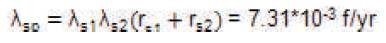
Therefore, the equivalent failure rate of the system is:

 

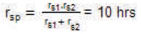
The mean outage time of the system is:

 

Hence, the average annual outage time of the system is:

 

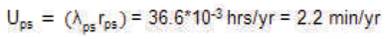
Consider that there are two components in a parallel configuration each having a failure rate of 0.2 f/yr and repair time of 20 hrs respectively and having such two parallel configurations to be connected in series having same failure rates and repair times of components. The basic probability indices of the system can be obtained as follows:

Here n=3;  m=2;  λ_p11 = λ_p12 =0.2 f/yr;  r_p11 = 20 hrs;  r_p12 = 20 hrs

Now, the equivalent failure rates of the parallel configurations are:

 

The mean outage times of the parallel configurations are:

 

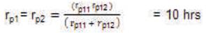
Therefore, the equivalent failure rate of the system is:

 

The mean outage time of the system is:

 

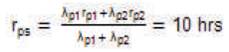
and the average annual outage time will be

 

Thus, for the same number of components, failure rates and repair times of the system, it has been observed from the above examples that,

• The equivalent failure rate decreases from unit redundant configuration to component redundant configuration
• Mean outage time is constant for unit and component redundant configurations
• The Average annual outage time decreases from unit redundant configuration to component redundant configuration, i.e., average annual operating time will be more for component redundant configuration as compared to unit redundant configuration
• Thus, it can be concluded that, component redundant configuration will be better than unit redundant configuration.

In the previous section, series, parallel, series-parallel, parallel-series configurations of systems have been considered for evaluating basic probability indices. For non-series-parallel configurations, some additional approaches are required. The reliability analysis of various systems using graph theoretic techniques have been dealt with path based and cutset based approaches. In particular, for any system which is represented by graph, cutset approach is very much suitable for approximate system reliability analysis as each cutset will also represent the failure mode of the system. Further, the elements in a cutset are considered in parallel and each such cutset is considered to be in series from the Reliability Logic Diagram point of view. Thus, it requires parallel-series configurations to be represented for evaluation of basic probability indices. In the previous section, parallel-series configuration has been shown to be the one with respect to component redundancy problem wherein each parallel configuration has same number of components connected. However, with respect to cutsets, although parallel-series configurations can be used, the number of elements in each cutset need not be unique. Thus, from the cutset algorithms, the cutsets of systems that represent failure modes of the system can be obtained and these cutsets will be inputs for evaluating basic probability indices of systems. Therefore, in this Section, the expressions for basic probability indices of system based on cutset approach will be derived. Consider the parallelseries configuration using cutsets as shown in Figure 3 (a) and the corresponding simplifications in Figure 3 (b) and ( c) respectively.

Let C₁₁ , C₁₂ , ..., C_1m be the components of 1st cutest; C₂₁, C₂₂ , ..., C_2m . are the components of 2^nd cutset.

C_n1 , C_n2, ..., C_nm. are the components of n^th cutset of a system.

Here 'n' is number of cutsets of the system.

m₁ , m ₂, . . , m_n are the number of elements of cutsets 1 to m respectively.

Thus, the basic probability indices can be evaluated as follows.

Let λ_cij be the failure rate of the j^th component of I^th cutest; r_cij be the repair time of the j^th component of I^th cutset.

Let λ_ci be the equivalent failure rate of the I^th cutest; r_ci be the mean outage time of the i^th cutset.

Let λ_cs be the equivalent failure rate of system; r_cs be the mean outage time of the system.

U_cs be the Average annual outage time of the system.

The mean outage time rci can be written as:

[25]

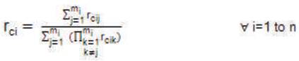
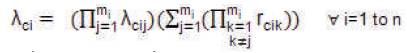
The equivalent failure rate λci can be written as:

[26]

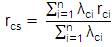
λcs can be expressed as:

[27]

Mean outage of the system rcs can be expressed as :

[28]

and the average annual outage time Ucs of the system can be expressed as:

[29]

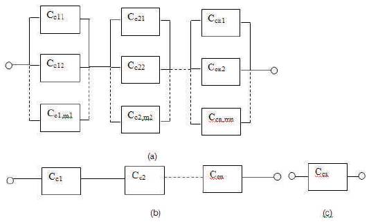
Figure 3. Parallel-series configuration of any system using cutset approach in (a) and corresponding simplifications in (b) and ( c)

In general, it is well known that Power System Network is treated as multi input multi output network with buses, where generators are connected as inputs, the buses, where the loads are connected as outputs. In the analysis of Power System Network reliability studies, various Cutset definitions are proposed [7].

However, as stated in the previous sections, no attempt has been made to generalize for any network to compute basic probability indices. As applied to Power Systems, the output Cutsets can be referred to as load point Cutsets, wherein there is no possibility of transmission to the load bus from any of the generator buses. Ideally, Power supply is to be ensured to all the load buses in the Power System Network. In this context, as applied to Power Systems, System Cutset implies that there is no possibility of transmission to any of the load buses from any of the buses where generators are connected. System Cutsets can be deduced from all load point Cutsets. The union of all the load point Cutsets will be system Cutsets. A sample 6 bus Roy Billinton Test System (RBTS) [1] considered is shown in Figure 4, which has 2 generator buses connected at buses 1 and 2, Loads are connected at buses 2 to 6. Graph for 6-bus RBTS is shown in Figure 5.

Cutsets of Load point 2 are:

C₁ : 12, 13; C₂ : 3,2,7,13; C₃ : 3, 1, 6, 13; C₄ : 3, 4, 5, 13 C₅ : 3, 4, 8, 13 and Reliability Logic Diagram of Load point 2 is shown in Figure 6.

Cutsets of Load point 3 are:

C₁ : 12, 13; C₂ : 1,6, 2,7,13; C₃ : 3, 1, 6, 13; C₄ : 4, 8, 1, 6; C₅ : 4, 5, 1, 6 , C₆ : 3, 2, 6, 12, C₇ : 3, 4, 8, 12 C₈ : 3, 4, 5, 12 and Reliability Logic Diagram of Load point 3 is shown in Figure 7.

Cutsets of Load point 4 are : C₁ : 12, 13; C₂ : 8,2,7; C₃ : 1, 6, 2, 7; C₄ : 3, 1, 6, 13, C₅ : 4, 5, 2, 7; C₆ : 12, 3, 2, 7 and Reliability Logic Diagram of Load point 4 is shown in Figure 8.

Cutsets of Load point 5 are : C₁ : 12, 13; C₂ : 3, 1, 6, 13; C₃ : 1, 6, 2, 7; C₄ : 4, 8, 1, 6; C₅ : 3, 2, 7, 12; C₆ :3, 4, 8, 12 and Reliability Logic Diagram of Load point 5 is shown in Figure 9.

Cutsets of Load point 6 are : C₁ :9; C₂ : 12, 13; C₃ : 3, 1, 6, 13; C₄ : 1, 6, 2, 7; C₅ : 4, 8, 1, 6; C₆ : 3, 2, 7, 12; C₇ : 3, 4, 8, 12  and Reliability Logic Diagram of Load point 6 is shown in Figure 10.

Cutsets of 6-bus RBTS are : C₁ : 9; C₂ : 12, 13; C₃ : 8, 2, 7; C₄ : 1, 6, 2, 7; C₅ :3, 1, 6, 13; C₆ :3, 2, 6, 13; C₇ :4, 8, 1, 6; C8 : 4, 5,   1, 6; C₉ : 3, 2, 7, 12; C₁₀ : 4, 5, 2, 7; C₁₁ :3, 4, 5, 13; C₁₂ : 3, 4, 8, 13; C₁₃ :3, 4, 8, 12; C₁₄ : 3, 4, 5, 13 and Reliability Logic Diagram of 6-bus RBTS is shown in Figure 11.

Generalized expressions given in Section 4 are applied to 6-bus RBTS by using MATLAB programming. The RBTS Branch and Generation data for three examples are given in Tables 1, 2, 4,5,7,8 and the basic probability indices are given in Tables 3, 6, 9 respectively.

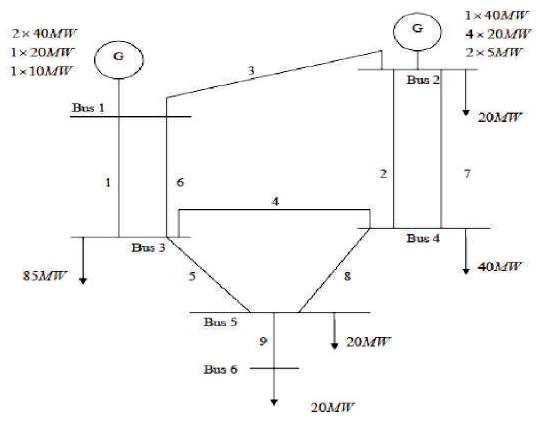
Figure 4. 6 bus RBTS

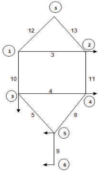
Figure 5. Graph for 6-bus RBTS

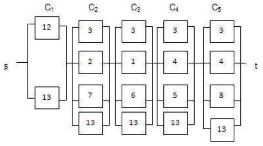
Figure 6. Reliability Logic Diagram of Load point 2 in 6-bus RBTS using cutset approach

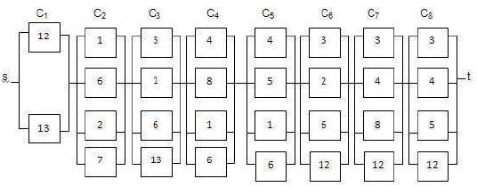
Figure 7. Reliability Logic Diagram of Load point 3 in 6-bus RBTS using cutset approach

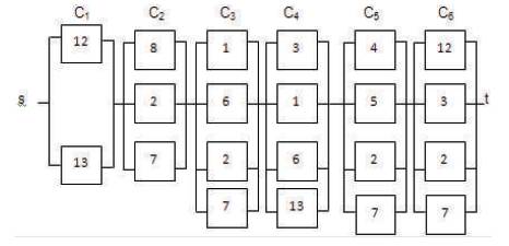
Figure 8. Reliability Logic Diagram of Load point 4 in 6-bus RBTS using cutset approach

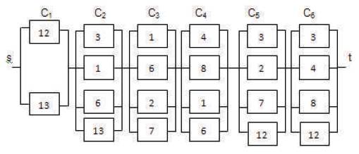
Figure 9. Reliability Logic Diagram of Load point 5 in 6-bus RBTS using cutset approach

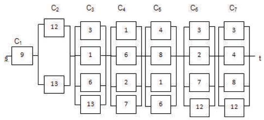
Figure 10. Reliability Logic Diagram of Load point

Figure 11. Reliability Logic Diagram of 6-bus RBTS using cutset approach

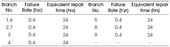
Table 1. Branch data of 6 Bus RBTS

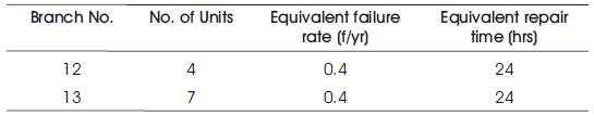
Table 2. Generation data of 6 Bus RBTS

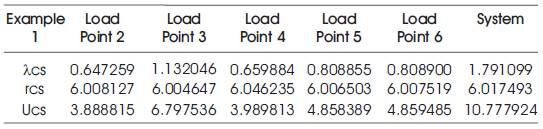
Table 3. Basic Probability indices for Example 1

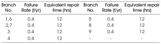
Table 4. Branch data of 6 Bus RBTS

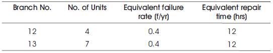
Table 5. Generation data of 6 Bus RBTS

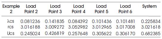
Table 6. Basic Probability indices for Example 2

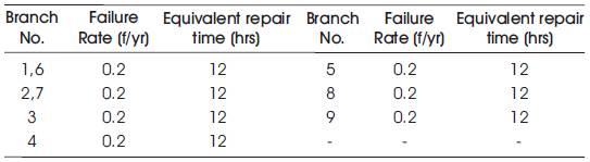
Table 7. Branch data of 6 Bus RBTS

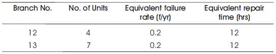
Table 8. Generation data of 6 Bus RBTS

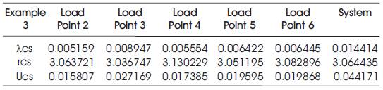
Table 9. Basic Probability indices for Example 3

From the above results the following conclusions can be made:

• As the number of cutsets are increased: λ_cs and U_cs are increased
• When r is reduced from 24 to 12 keeping λ_cs as constant, all equivalent parameters are decreased. (Examples 1 and Example 2)
• When λ is reduced from 0.4 to 0.2 keeping r as constant, and U_cs are decreased, r_cs is increased. Examples 2 and 3)

It is verified that component redundancy is better than unit redundancy configuration to improve the reliability of the system even for exponentially distributed failure rate of the components. The basic probability indices for the case of repairable systems with series, parallel, series- parallel, parallel- series and complex configurations are determined and several properties have been deduced based on these configurations. Application to Power System Networks has been dealt with using Cutset approach and basic probability indices of load point and of Power System Network are computed.

It has been observed that as number of Cutsets increase, equivalent failure rare and average annual outage time also increases. Further, as mean outage time is reduced, keeping failure rate of each component constant, all basic probability indices are reduced. Also, when failure rate of each component is reduced, keeping mean outage time as constant, equivalent failure rate and average annual outage time are reduced and equivalent repair time is increased. The proposed method offers enough approximated formulae to simplify large systems and also used in reliability evaluation and optimization calculations.