(1)

This paper discuss the different strategies which enable wind power market to enhance reliability to integrate competitive power grids economically. Wind mills are newly globalized techniques to the Restructured Power Systems that are difficult to schedule due to variability and un-predictability. Now a day's Wind energy is termed as Price Taker due to the issues like Transmission Congestions. Although Locational Marginal Pricing (LMP) plays an important role in many restructured wholesale power markets, the detailed derivation of LMPs as actually used in industry practice is not presently available. This paper demonstrates these problems by two sections. Firstly, the overview, definitions, characteristics, settlements, observations and examples for the Locational Marginal Prices or LMPs for particular generators that are developed on the basis of congested and uncongested case. Secondly, calculation for AC and DC optimal power flow models. Wind energy generation system for Restructured Power Systems is simulated using MATLAB.
Now a day's Wind energy is termed as Price Taker due to the issues like transmission congestions, energy cost, transmission loss cost. The wind power is one of the oldest renewable technologies, which converts kinetic energy of wind into mechanical or electrical energy. Due to the convective nature processes due to temperature differences to air motion wind energy produced and are vary from different altitudes on the earth [1]. Hence the selection of site for measuring the wind energy for the required speed is very difficult because of its variable characteristics. Even though the weather conditions may cause the measured wind energy to be not constant we can adjust the speed to be equal to the required efficiency by changing the height of the tower [2].
A wind mill is newly globalized techniques to the Restructured Power Systems but is difficult to schedule due to variability and un-predictability because of its intermittent nature (wind always does not blows). Globally, the installed wind energy capacity is over 157,900 MW. India today has the fifth largest installed capacity of wind power in the world with 11087MW installed capacity and potential for on-shore capabilities of 65000MW. According to the Global Wind Energy Council, around half a million people are now employed by the wind industry around the world.
Obviously, based on the different locations the marginal prices are varying but these problems can be rectified by Locational Marginal Prices which is used for the calculations for the next incremental costs and defined as the marginal cost to serve one More Megawatt (MW) of load at a certain location [3]. Wind farm developers are investigating potential wind farm sites throughout our world. This proposed energy is not affecting any kind of imbalance in emissions and achieves energy security; many governments are turning to tax relief to promote renewable energy sources for power generation. When the generator at a specific location is causing economic harm to the entire system, adding one more MW of load may have somewhat counterintuitive effects.
Most of the references have described the wind power production as a money taking power plant after Solar power plant. Thus the lack of solution in the variability, unpredictability and correlated behaviour of wind farms resulted in the increased usage of Solar Panels and Hydro power plants. It is proved that Wind Turbines are securing more land for constructions other than Wind Plants. The work presented by Jónsson et al. proved that wind power behaves as a price maker in electricity markets. El-Fouly et al. develop the wind production on market prices and total generation costs [4]. The main contribution of this paper is to equate the supply and demand of producers and consumers in an electrical power market with the detailed explanation for LMPs.
The problems affecting the wind power markets, like transmission congestion Pricing can be solved only by the detailed derivation of LMPs and the economic limitations for the operation of wholesale power markets. This will result in the impromptu situation for wind producers due to the misjudging of MWh prices. In this paper, the detailed explanation of restructured power markets is solved on the presence of transmission limits. In Section 1 the concept, calculation and practical application of LMPs and in Section 2 presents, Economics of power generation of restructured power system for the consumer demand and production supply are presented. In Section 3, the calculations for Transmission Congestion Costs based on the Uplift Charges, System Redispatch Payments and Congestion Revenues examining the calculation for LMPs as an example of 3-bus system when one bus is subjected to a load obligation is given. Section 4 concludes the paper.
The definition and calculations of LMPs depend upon economic theory and power system, when the transmission congestion affects the cost of generations and lowering the market benefits [5]. The word LMP is used as a building blocks for the accurate calculation for Transmission Prices. The Marginal Cost can be explained only by designing a system with the similar total system cost and transmission end cost or by maximizing the social welfare (difference in demand and production).
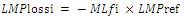
Objective function is calculated by maximizing the demand offer and supply bid. This is subject to the constraints by the presence of transmission limits and line losses. The LMPs or nodal prices are the combination of three components: marginal cost at a reference bus, marginal cost of transmission losses, and marginal cost of transmission system congestion.
The LMP (nodal price) at Bus i can be calculated using the following equation:
Nodal Price Components:

The marginal cost of losses from the ref- bus to bus i:
The marginal cost of losses from bus i to the ref- bus:

To keep a power balance, the injection at bus i will be,

- MLf is termed as positive if there is an increase in losses I and as negative if there is a decrease in losses.
Marginal cost of transmission congestion from the reference bus to bus i:

Marginal cost of transmission congestion from bus i to the the reference bus:

This is the incremental change in the system cost over an incremental change in the constraint limit.
The charge for selling 1 MW at A and buying 1 MW at B are (neglecting losses) exactly the same as the charge for transmission from A to B.


The rate for transmission from A to B is the congestion rate and is priced at:

Transmission service for bilateral transactions is shown on the case study which explains the load and supply based on economic dispatch.
For many decades, vertically integrated electric utilities monopolized the way they controlled, sold and distributed electricity to customers in their service territories. In this monopoly, each utility managed three main components of the system: generation, transmission and distribution [6]. A competition is guaranteed by establishing a restructured environment in which customers could choose to buy from different suppliers and change suppliers as they wish in order to pay market-based rates. The main objective is the reduction of cost which is achieved by ensures competitions and guarantee choice to the customers for selection based on the greater incentives of short and long term efficiencies than economic regulations.
FERC Order 888 required transmission owners to provide a comparable service to other customers who did not own any transmission facilities and developed eleven principles for restructuring electrical industry [7]. The primary objective of ISO is not dispatching or redispatching generation, but matching electricity supplies with demand as necessary to ensure reliability. Power Exchange (PX) accepts supply and demand bids to determine a MCP for each of the 24 periods and ISO should control generation to the extent necessary to maintain reliability and optimize transmission efficiency.
The condition where overloads in transmission lines or transformers occur is called congestion. Congestion may be prevented to some extent (preventive actions) by means of reservations, rights and congestion pricing. Also, congestion can be corrected by applying control (corrective actions) such as phase shifters, tap transformers, reactive power control, redispatch of generation and curtailment of loads [9]. Congestion could prevent system operators from dispatching additional power from a specific generator. Electricity is a non-storable commodity and its supply and demand must be matched at all the times. Price Volatility is a measure of instability in future prices or uncertainty in future price movements. Volatility is directly proportional to standard deviation [10]. Customers use the concept of elastic demand when they are exposed to and aware of the price of energy.
When we are been inside the economics, it is very important to find the several factors which influence the production cost such as cost of land and equipment, interest on capital investment etc. Therefore, a careful study with different steps are founded in this section with various parts including depreciation charge, capacity factor, load factor, interests and annual cost production calculations [11]. The total annual cost of electrical energy generated can be divided into three parts and two parts systems,
For three part systems: CT=Rs(Fc+SFc+Rc) or
For two part systems: CT=Rs(AKW+BKW)
Constant which when multiplied by maximum KW demand on the station gives the annual cost (A) and when multiplied by the annual KWh generated gives the annual running cost (B).
In the Straight line method, Annual depreciation charge (Adc) is the ratio of Total depreciation (Td) and Useful time (Ul).

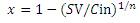
In the Diminishing value method:
Value of the equipment after 'n' year = Cin (1-x)n
Value of the equipment after n years is the difference between the diminished value and annual depreciation.
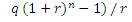
In the Sinking fund method:
Cost of replacement= Cin-SV
Amount q deposited at the end of first year becomes:

Annual deposit in the sinking fund is,

Sinking fund at the end of n years:
The load factor plays a vital role in determining the cosy of energy and is calculated by average load over maximum demand. Some importance advantages of high load factor are the reduction of unit generated and variable load problems.
Average load = Area (in KWh) under daily load curve
24 hours
Unit generated per annum:
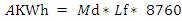
Annual Running Charge (ARC) for a power plant is the combination of annual cost of fuel and taxes, wages but for wind (Arc is without the cost of fuel and oil). Annual fixed cost is the percentage of interest and depreciation with respect to the capital cost, life time, interest and loans.
Capacity factor is the ratio of actual output (Average demand) and total expected output (Installed capacity),

Total annual operating cost of station A and B:
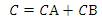
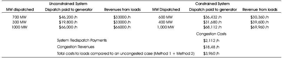
Table 1. Dispatch, dispatch costs, and revenues for the unconstrained and constrained systems
The size of a generator can be easily calculated by the calculation of annual energy production cost, hence capacity factor can be assumed to be 20-50% and the availability of turbine is 90-98%. AEP is the product of expected power, availability and the time.

When we are implementing the expected parameters of a particular wind mill in the above equations, it can be calculated that: the site which is working at high wind speed (15m/s) for a period of half an year is more efficient than a site with an entire year working capability with 7m/s [12].
This section gives the detailed calculation for examining the calculation for LMPs in a two area networks as an example based on a constrained system and unconstrained system [13]. In this example, the real time price for wind power in Tamilnadu state (largest wind power potential state in India) ($0.066/kWh) is taken as an example and it will be of $66/MWh.
Firstly, system redispatch payments can be calculated by taking the difference of un-congested case (product of supply and cost per MWh) and congested case (product of supply and cost per MWh). Here, congestion cost is equal to change in dispatch order. Secondly, congestion revenue can be calculated by finding the difference of congested case (product of fixed load and changed cost) and congested case (product of supply and cost) [14-16].
In Table 1, first column represents the Area A, second Area B and third Total respectively.
Uplift Charge can be found by finding the product of congested supplies with uncongested cost and transmission limit supply with increased transmission cost [17]. Here, the congestion cost is the dispatch payments out of merit order. In the restructured market, the Uplift charge can be calculated by,
(600*66) + (300*66) + (100*72.6) = $66660/h
The combined energy and Uplift cost price to the load can be calculated by,
66660/1000=$66.66/MWh
The additional transmission capacity results in an LMP change in Area A from $60.72/MWh(congested) (Figure 2) to $66 /MWh (uncongested) and from $79.20 /MWh (congested) to $66 /MWh (uncongested) in Area B (Figure 1).
With an increase in transmission capacity, production in Area A increases from 600 MW to 700 MW, and the price increases linearly from $60.72 /MWh to $66 /Mwh.
In the above network in Figure 3 it is no transmission limit and hence the flow is uniform (only needed supply is taken).
In the above network in Figure 4 it is a transmission limit so we re-dispatch the power flow. The calculation for line losses are calculated easily by taking the product of actual and final flow.
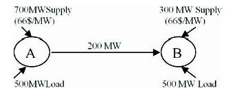
Figure 1. Two Area Network (Un-Congested Case)
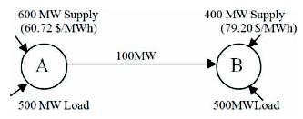
Figure 2. Two Area Network (Congestion Case)
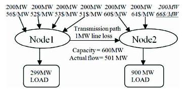
Figure 3. Two Nodes System (No transmission constraints)
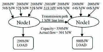
Figure 4. Two Nodes Network (transmission constraints)
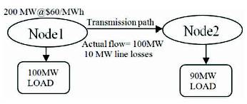
Figure 5. Two Nodes Network (with line losses)
In Figure 5 line losses are included and it causes the increase in price without Congestion. Hence, node 4 price can be calculated by, (Price in node3 ($) * actual flow (MW)) / node 4 = ($60/MWh*100MW)/90 MW= $66.66/MW.
In a system, the ghastliest situation that is found is the transmission congestion circumstances which are more hazardous to entire buses [18]. Marginal Clearing Prices (MCP) can be calculated by the multiple points around a system which is known as a node. A node is a point where supply enter into a system such as a generator bus bar or transmission inter-tie or the supply given out such as distribution substations [19-20]. The prices under the integrated model are called Locational Marginal Pricing or Nodal Pricing which are calculated at each node on the system.
In the case without load obligations G1 can supply the entire load. When the system is under transmission limits (load obligation in G2), the contingency analysis is used to ensure security [21]. Firstly, adding one MW of load to bus 1, this can easily be supplied by G1 which causes no serious change. Secondly, adding one MW of load to bus3 (Figure 6), the transmission system is congested and no more power is available from G1 [22-23]. Finally, by adding one MW of load to bus2 counter flows can be achieve by reducing 1MW in the bus 3 and flows from bus1-2 and bus 3-2.
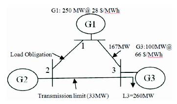
Figure 6. 3-bus system with Transmission limit
In Table 2 the columns shows the base case, adding 1MW to bus1, bus3, bus 2 respectively. In the Table 3G3MW is assumed to be zero. Hence, G3MW*G3 Cost is assumed to be zero.
Table 3 shows the economic Curtailment in which, the high cost wind supply is turned off [21-23].
Figures 7-9 show the simulation results.
From the above results, it is shown that the correlation among wind farms has an important effect on LMPs, especially on their volatilities and if the network becomes congested, the wind impact on LMPs becomes local. Wind production reduces the electricity price, but increases its volatility [24]. High wind power penetration levels increase the frequency of zero-price events, which is in accordance with empirical results. The amount of wind power being added into many power systems is increasing dramatically (Figures 7 and 8). This increase requires a similar increase in the amount of transmission capacity to be able to supply many loads with low-cost energy.
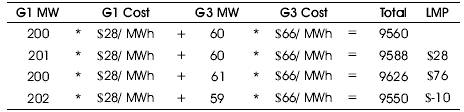
Table 2. Costs and Prices without Economic Curtailment
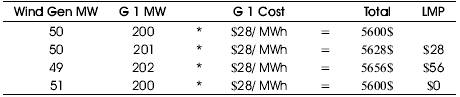
Table 3. Costs and Prices with Economic Curtailment
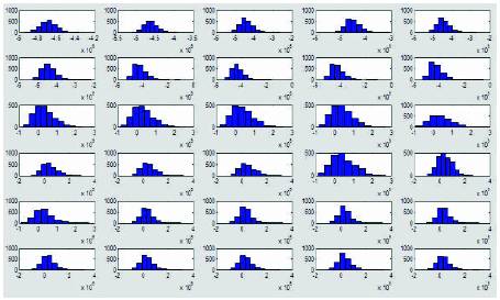
Figure 7. Un-congested System (supply and load are linear) and Congested system (supply and loads are varying)
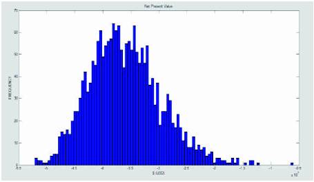
Figure 8. Uplift Charges and Calculated Values for line losses
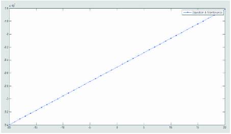
Figure 9. Cost with Economic Curtailment
This paper provides a detailed explanation for the economics calculations and an easy methodology for the overall cost calculations for the Wind mills. In the above calculations, the authors calculated congestion in a restructuring market and line losses which can affect the entire systems. For maximizing the Social Welfare, the LMPs for different locations with line losses, congestions and economic curtailment are calculated. Most of the problems regarding Wind power markets in the present conditions are solved with the help of two area networks and three bus systems. Firstly, the authors calculate the economics of wind power market including the overall parameters. Secondly, the LMPs are calculated on the basis of constrained and Un-constrained system based on two node systems with different supplies and demand. Finally, above calculations are simulated on the basis of consumer and producer surplus.
In the final MATLAB result, it is shown that without transmission limits, curves are linear and otherwise nonlinear. As future works we intend to implement in IEEE 24 BUS System.
The notations used throughout in this paper are stated below for quick reference:
| LMPi | Nodal price(LMPs) at bus |
| LMPref | Nodal price at the reference bus |
| LMPLossi | Marginal cost of losses from reference bus to busi. |
| LMPCongestioni | LMP in transmission congestion. |
| MLfi | Marginal loss factor at bus I |
| Ii | Injection at bus I |
| Tlosses | Transmission losses |
| Spj | Shadow price of constraint j |
| Sfj | Shift factor for real load at Bus i on constraint j |
| CT | Total annual cost of energy |
| Adc | Annual depreciation charge |
| Fc | Annual fixed cost independent of maximum Demand |
| SFc | Annual semi fixed cost multiplied by Maximum, ( KW) |
| Rc | Running or operating cost multiplied by Kwh |
| Td | Total depreciation |
| Ul | Useful life of the equipment |
| AKWh | Annual energy production, kWh/yr |
| AEP | Annual Energy Production, kWh |
| Lf | Load factor |
| Cf | Capacity factor |
| Ta | Turbine availability (depending upon the construction) |
| Gs | Generator size (rated power), kW |
| Cin | Initial value or capital cost |
| Lf | Load factor |
| Sv | Scrap value after useful life |
| n | Useful life of the equipment in years |
| r | Annual rate of interest expressed as a decimal |
| Md | Maximum demand |
| Arc | Annual running charge |
| Ad | Average demand |
| Ic | Installed capacity |
| x | Annual unit depreciation |
| q | Amount of depreciation every year. |