Medical images are often low contrast images and they employ a complex kind of noise due to various acquisitions, transmission storage space and screen devices. Also they involve the application of unique variations of quantization, reconstruction and enhancement algorithms. All medical photographs contain visible noise. The existence of noise gives the photo a mottled, grainy, uneven or arctic appearance. Image noise originates from a range of sources. No image resolution method is without any noise, but the noise is quite a bit more prevalent in certain types of imaging processes than the others. Nuclear images are likely to be one of the noisiest. Computed Tomography (CT) and Magnetic Resonance Image (MRI) resolution will be the two modalities which can be regularly used for brain image resolution. CT image resolution is recommended over MRI due to lower price, short image resolution times, common availability, simple access, maximum detection connected with calcification as well as hemorrhage, and finally an excellent solution of bony aspect. CT tests of bodily organs, bones and soft tissues provide increased clearness compared to conventional X-Ray. Nevertheless, the limitations for CT checking of head images are a result of partial level effects that affect the edges along with lower brain muscle contrast[1]. CT is really a radiographic examination method, which generates some sort of 3-D image from the inside part of the object from the large number of 2-D images taken on across sectional plane from the same target. CT creates thin slices from the body that has a narrow X-Ray, which rotates around the body of a stationary individual [2].

Additionally, noise could be introduced simply by transmission errors and data compression[3]. So, it is necessary to make use of a productive denoising method to compensate this kind of data file corruption error. Image denoising, nonetheless, remains difficult because noise removal highlights artifacts and also causes blurring on the images. This paper describes diverse methodologies intended for noise decline or denoising giving an insight about which algorithm ought to be used to search the most trusted estimate on an original photograph length information, given its degraded type. Sound modeling within images are usually greatly troubled by capturing equipment, data tranny media, graphic quantization and the discrete solutions regarding radiation[4]. Different algorithms are utilized with regard to the noise design. Most of the natural photographs are assumed to have additive hit-or-miss noise which can be modeled being a Gaussian.

Throughout the last decade, there has been various involvement in wavelet techniques for noise eradication in indicators and images. The fundamental steps include easy ideas like thresholding from the orthogonal wavelet coefficients from the noisy data, followed by reconstruction. Later, large improvements throughout perceptual excellence were acquired by interpretation invariant methods according to thresholding of the undecimated wavelet alter. Recently, tree-based wavelet de-noising strategies were developed inside contexts regarding image de-noising, which exploit the sapling structure of wavelet coefficients and the so-called parentchild correlations, which might be present throughout the wavelet coefficients of images having edges. Consequently, many researchers have experimented with variations within the basic schemes, and modifications involving thresholding characteristics, leveldependent thresholding, prevent thresholding, adaptive selection of threshold, Bayesian conditional requirement nonlinearities etc, [5] [6].

An exclusive member with the emerging class of multiscale geometric transforms would be the Curvelet transform which has been developed in the last few years, so as to overcome the built-in limitations of the traditional multistage representations such as wavelets. The Curvelet enhance like the particular wavelet enhance, is a multiscale enhance, with body elements listed by degree and spot parameters. The enhance was built to represent edges and other singularities along curves, a lot more efficiently compared to traditional converts like electronic noise Numerous small coefficients were used for the given accuracy and reliability of reconstruction. Thus, in order to represent an advantage to squared error, 1/N involves 1/N wavelets and only about 1/√N curvelets [7-11].

Image noise is a random (not within the subject images) variant of perfection or color information throughout the images, and it is usually an aspect of electronic noise. It is usually produced from the sensor as well as the circuitry of a scanner or camera. Image noise could also originate through film wheat and from the unavoidable noise of an ideal photon detector. Image noise is usually an undesirable by-product involving image size that contributes spurious as well as extraneous information. The unique meaning involving "noise" has been staying as "unwanted signal"; unwanted electrical movement in signals received by AM radios induced audible acoustic noise ("static"). For example, unwanted electric powered fluctuations themselves came to be known seeing that "noise". Image noise is a program, which is[1] inaudible. The magnitude of photograph noise can consist of almost imperceptible specks on the digital photograph used for good lighting, from optical to radio astronomical images, which might be almost fully noise, from which a tiny bit of information may be derived by sophisticated processing (a sound level that is totally unacceptable in a photograph since it might be impossible to view even what the topic was).

Nguyen Thanh Binh and Ashish Khare presented new adaptive techniques depending on Curvelet enhance using cycle spinning intended for de- noising. It removes the signal based mostly on noise for instance speckle sounds. It is clear that, in almost too many cases, each of the proposed procedure performs better than the various other methods. The biggest problem using image denoising is shift- sensitivity. By carrying out cycle spinning, the best error of a denoised impression is reduced, producing lower energy from the error which provides better denoising consequence. This is amongst the reasons precisely why our proposed method performs better than the various other methods[12].

Tanjeet Kaur, Gaurav Gupta, Gagandeep Kaur suggested Curvelet Transformation based photograph denoising, which is along with Gabor filter instead of the minimal pass filtering from the transform sector. For minimal noisy photos, Translation invariant wavelet primarily based method also provides better final results, but for the reason that the noise increases, all Curvelet primarily based methods outshine the wavelet primarily based methods. An optimized Gabor filter is needed to attain edge recognition of accurate parts, and acquires precise edge features by way of a reasonable alternative to way and level [13].

G. Mamatha and L. Gayatri presented the latest trend inside fusion associated with digital picture, MRI, and also CT graphics which depends on the Curvelet enhance. An assessment study has been made between the traditional wavelet blend algorithm and the proposed Curvelet blend algorithm. The experimental study shows that, the application of the Curvelet transform inside fusion associated with MR and also CT graphics is of finer quality than the application of the conventional wavelet enhance. The received Curvelet blend resulted in higher connection coefficient and the entropy prices than inside wavelet blend results and also minimum prices of RMS error than inside wavelet enhance. Finally, these blend methods are used in simulation findings of multi-focus and also complementary blend images. With vision, the blend algorithm proposed in this paper acquires a better blend result. With an objective examination criteria, Curvelet blend characteristics have finer quality than traditional DWT[14].

Sweta Mehta and Bijith Marakarkandy put forward an image fusion algorithm based on Wavelet Transform and Curvelet Transform. It provides a multi resolution analysis ability in Wavelet Change, which also possesses a better way of identification ability to the edge element of the awaiting described images within the Curvelet change. This procedure could describe the edge way of photos, and analyzes the feature of images greater. MRI impression provides a greater comparison between various soft fleshes of human body than a CT impression. Brightness of bones is higher for CT photos but, delicate tissues cannot be seen. Fusion impression provides an equal characteristics of CT and MRI within a single impression [15].

P. Karthikeyan, S. Rama Subramanian, G. Rajasekaran, S. Musafar Rafee explained numerous properties, respected through the Curvelet coefficient. The superior images on the modified Curvelet coefficients were restored. Noise ought not to be amplified throughout enhancing edges. The enhanced image is reconstructed on the modified Curvelet coefficients. It is quite advantageous in case of block effects, which usually do not occur. Block overlapping is often not essential in comparing Curvelet-based enhancement. The Curvelet improvement functions consider an account adequately for the photograph noise. As evidenced through the experiments while using the Curvelet enhance with wavelets, there exists a better diagnosis of raucous curves compared with other methods [16].

Image de-noising can be a vital impression processing job. As a task, in addition to a component inside other procedures, there are usually many approaches for denoising a graphic or a set of data in addition to the methods out there. The significant property of a good impression denoising design is that, it should entirely remove noise as far as possible as well as preserve the ends. Traditionally, two forms of models i.e. linear design and non-linear design were found. Generally, linear models were used. The advantage of the linear disturbance removing models will be the speed and the limitations from the linear designs is that, the models cannot preserve edges from the images in an efficient manner. The ends, which are acknowledged as the discontinuities from the image, are usually smeared out. On the other hand, Non-linear models can handle edges in a much better way than the linear designs. One well- known model with regard to a non-linear impression denoising will be the Total Deviation (TV) filter. In order to de-noise, a new degraded impression X is given by, X = S + N, where S will be the original impression and N can be an Additive Whitened Gaussian disturbance with mysterious variance [2].

Sounds reduction is the process of removing noise from your signal. Many recording products, both analog and digital, have traits which make them susceptible to noise. Noise could be random or white noise with no coherence or coherent sound is introduced with the device's mechanism or the running algorithms. In electronic devices, an essential form of noise is actually hiss attributable to random electrons that are heavily swayed by high temperature, and strayed from their designated path. These wayward electrons effect the voltage with the output signal and therefore create a detectable sound. In the situation of photograph taking film along with magnetic tape, noise (both seen and audible) is actually introduced because of the grain structure with the medium. In photographic motion picture, the size of the grains within the film decides the film's tenderness, more vulnerable film possessing larger type of grains. In magnetic tape, when the grains with magnetic allergens (usually oxide or magnetite) are bigger, the medium is more prone to noise. So, larger parts of film or magnetic tape enable to lower the noise to an acceptable level.

The actual Curvelet transform is a higher dimensional generalization from the Wavelet transform built to represent photos at different scales and different angles. Curvelets take pleasure in two distinctive mathematical houses.

Curved singularities may be well approximated with a small number of coefficients and inside a non-adaptive approach, hence the actual name, "Curvelets". Curvelets remain as coherent wave forms under the actual action from the wave equation inside a smooth method. Curvelets can be a non-adaptive technique for multi scale target representation. As an extension from the wavelet strategy, they are becoming popular inside similar grounds, namely inside image finalizing and methodical computing. Curvelets are in a proper basis regarding the representation of photos (or some other functions) which is smooth, as well as the singularities combined smooth figure, where the actual curves have bounded curvature, where the objects inside the image employ a minimum size scale.

That property supports for cartoons and geometrical diagrams, in addition to text. United zoom on such images shows that the actual edges they contain show up increasingly right. Curvelets benefit from this residence, by defining the more expensive resolution Curvelets being skinnier than the fewer resolution Curvelets. Nevertheless, natural photos (photographs) will not have this residence; they get detail with every size. Therefore, based on the natural photos, it surpasses the use of getting some sort of directional wavelet convert, whose wavelets possess the same facet ratio with every size. Curvelet Transform gives a superior overall performance in image denoising as a result of these properties, for example, scarcity in addition to multi resolution design. For a CT, in addition to medical photos, the information ought to be refined with regard to better technique, so that the radiologist could give a better opinion for your diagnosis.

4.1 Curvelet transform based denoising

These Curvelets are based on multi-scale formlets combined with a spatial band pass filtering operation. These band pass filtration systems are set so that the Curvelet length and the width are at a normal scale, which observe the climbing rule size length as 2. A 2-D wavelet transform is employed to isolate the graphic at which the unique scale, in addition to spatial partitioning, is employed to break each scale into prevents. Large size blocks are employed to partition large scale wavelet change components to small size blocks which are employed to partition small scale parts. Finally, the form let change is placed on each prohibit. By using this method, the graphic edges in a certain scale are usually represented efficiently by the ridge allow transform as the image perimeters are pretty much like right lines from that scale. The Curvelet change can sparsely define the high dimensional signals that are fitted with lines, figure or hyper airplane singularities.

The normal processes of the digital realization for Curvelet transform consist of these four phases:

1) Sub-band Decomposition
Dividing the graphic into decision layers. Each covering contains details of different frequencies:
P_o –Low-pass filtration.
Δ1, Δ2, Applying Log Gabor filtration to approx. the frequencies.
The original image can be reconstructed from your sub-bands, so sub-band decomposition has to be performed.
2) Smooth Partitioning
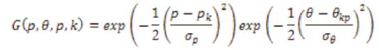
The actual windowing operate w is a nonnegative smooth function.
3) Renormalization
Renormalization is actually centering every dyadic square on the unit block, [0, 1]× [0, 1].
For every Q, the operator TQ is actually defined, prior to the Ridgelet Change. The A_sf layer contains objects using frequencies near the domain .
4) Ridgelet Analysis Every normalized block is analyzed inside the ridge allow system. The shape fragment possesses an  aspect ratio of 2^-2s ×2^-s . Following the renormalization, it offers localized consistency in wedding band  [2^s , 2^s+1 ]. A shape fragment needs only a handful of ridgelet coefficients to represent that.

Medical images are generally of low contrast and they often have a complex type of noise due to various acquisitions, transmission storage and display devices and due to the application of different types of quantization, reconstruction and enhancement algorithms. All medical images contain visual noise. Image de-noising is a vital image processing task, as a process itself and as a component in other processes. There are many ways to de-noise an image or a set of data and methods that exist. The important property of a good image denoising model is that, it should completely remove noise as far as possible and should preserve edges. Curvelets are a non-adaptive technique for multiscale object representation. Being an extension of the wavelet concept, they are becoming popular in similar fields in image processing and scientific computing. Curvelet Transform gives a superior performance in image denoising due to properties such as scarcity and multiresolution structure. For the CT and medical images, information need to be refined in a better way, so that the radiologist could give a better opinion for diagnosis. In this paper, we proposed a technique or a compression in which we used several number of image noise estimators. Estimator estimates the noise in the given image and put this estimation and the noisy image to Curvelets transform as shown in Figure 1. Figure 2 shows various phases of Curvelet Transform. Figure 3 shows how noise is estimated. In this paper, we present a comparison of various noise estimators with the Curvelet transform as an efficient denoising technique. The following were used as the estimators.

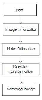
Figure 1. Proposed Methodology Flow Chart

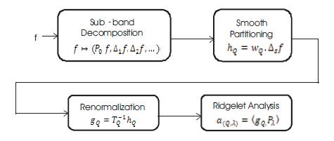
Figure 2. Curvelet Transform

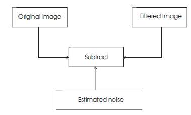
Figure 3. Noise Estimation Using Filter

5.1 Gabor Filter

Gabor filters are commonly recognized as one of the best choices for obtaining localized frequency information. They offer best simultaneous localization of spatial and frequency information. There are two important characteristics of Log-Gabor filter. Firstly, Log-Gabor function has no DC component, which contributes to improve the contrast ridges and edges of images. Secondly, the transfer function of the Log-Gabor function has an extended tail at the high frequency end, which enables to obtain a wide spectral information with localized spatial extent and consequently helps to preserve true ridge structures of images. The Gabor filter bank is a well-known technique to determine a feature domain for the representation of an image. However, a Gabor filter can be designed for a bandwidth of 1 octave maximum with a small DC component in the filter. A Log- Gabor filter has no DC component and can be constructed with any arbitrary bandwidth. There are two important characteristics in the Log-Gabor filter. Firstly, the Log-Gabor filter function always has zero DC components, which contribute to improve the contrast ridges and edges of images. Secondly, the Log-Gabor function has an extended tail at the high frequency end which allows it to encode images more efficiently than the ordinary Gabor function. To obtain the phase information, Log-Gabor wavelet is used for feature extraction. It has been observed that, the log filters can code natural images better than Gabor filters. Statistics of natural images indicate the presence of high-frequency components. Since the ordinary Gabor filters underrepresent high frequency components, the log filters are a better choice.

(1)

5.2 Variance Noise Estimation

A novel algorithm for estimating the noise variance of an image is presented. The image is assumed to be corrupted by Gaussian distributed noise. The algorithm estimates the noise variance in three steps. At first, the noisy image is filtered by a horizontal and a vertical difference operator to suppress the influence of the (unknown) original image. In the second step, a histogram of local signal variances is computed. Finally, a statistical evaluation of the histogram provides the desired estimation value. For a comparison with several previously published estimation methods, an ensemble of 128 natural and artificial test images were used. It is shown that, with the novel algorithm, more accurate results can be achieved using real CCD camera noise, which is not simply additive; it is strongly dependent on the image intensity level. The noise level is a function of image intensity, which is the Noise Level Function, or NLF. Since it may not be possible to find image regions at all the desired levels of intensity or color, the noise level function needs to be described.

5.3 Median Filtering

Median filtering is a nonlinear method used to remove the noise from images. It is widely used, as it is very effective in removing noise while preserving the edges. It is particularly effective at removing 'salt and pepper' type of noise. The median filter works by moving through the image, pixel by pixel, replacing each value with the median value of neighboring pixels. The pattern of neighbors is called the "window", which slides pixel by pixel over the entire image pixel of the entire image. The median is calculated by first sorting all the pixel values from the window in numerical order, and then replacing the pixel being considered with the middle (median) pixel value.

5.4 Low Pass Filter

A low pass filter can be as simple as an averaging function, in which a 'sliding window' average of some number of samples is calculated. The filter can be described in the frequency domain, for instance, it could th be a 4 -order filter with cut-off frequency of F . To filter the c input signal, the operation is performed either in time, or in frequency. The choice would depend on the type of filter, and the form of output required (time-domain or frequency-domain).

Convolution in time corresponds to Multiplication in frequency, and conversely, Multiplication in time corresponds to Convolution in frequency. If the filter is implemented as a time series (even the sliding window averaging filter is a time-series function), the input timedomain signal (sin 4t) is convolved with the filter timedomain transfer function. This is equivalent to multiplying the input frequency-domain signal with the filter frequency-domain transfer function. For simple filters, we can use the time-domain approach in Matlab. For more complex filters, the Signal Processing Toolbox to develop the filter transfer function is used, and then the filtering in time is done (using 'convolve' or frequency (using FFT, matrix multiplications, and IFFT) as needed.

5.5 Convolution Mean Filter

Image filtering allows to apply various effects on the photos. The type of image filtering described here uses a 2D filter similar to the one included in Paint Shop Pro as User Defined Filter and in Photoshop as Custom Filter.

Convolution

The trick of image filtering is that, it has a 2D filter matrix, and 2D image. Then, for every pixel of the image, the sum of products is taken. Each product is the color value of the current pixel or a neighbor of it, with the corresponding value of the filter matrix. The center of the filter matrix has to be multiplied with the current pixel, the other elements of the filter matrix with corresponding neighbor pixels. This operation takes the sum of products of elements from two 2D functions, where one of the two functions move over every element of the other function, which is called Convolution or Correlation. The difference between Convolution and Correlation is that for Convolution, the filter matrix has to be mirrored, but usually it is symmetrical and so there is no difference. The filters with convolution are relatively simple. More complex filters that can use more fancy functions exist as well, and can do much more complex things (for example, the Colored Pencil filter in Photoshop). The 2D convolution operation requires a 4-double loop, so it is not extremely fast, unless using small filters. Usually, we use 3x3 or 5x5 filters.

There are a few rules about the filter:

1) Its size has to be uneven, so that it has a center, for example 3x3, 5x5 and 7x7 are correct.
2) It does not have to, but the sum of all elements of the filter should be 1, if the resulting image wants to have the same brightness as the original.
3) If the sum of the elements is larger than 1, the result will be a brighter image, and if it is smaller than 1, it will be a darker image.
4) If the sum is 0, the resulting image is not necessarily completely black, but it'll be very dark.
5) In Mathematics and, in particular, functional analysis, convolution is a mathematical operation on two functions f and g, producing a third function that is typically viewed as a modified version of one of the original functions, giving the area overlap between the two functions as a function of the amount that one of the original functions is translated. Convolution is similar to cross-correlation. It has applications that include probability, statistics, computer vision, image and signal processing, electrical engineering, and differential equations. Convolution can be defined for functions on groups other than Euclidean space. For example, periodic functions, such as the discrete-time Fourier transform, can be defined on a circle and convolved by periodic convolution.

5.6 Weiner Moda

A new reconstruction method based on Wiener filtering of RF ultrasound echo signals has been presented. The algorithm takes into account the focusing effects of a transducer, frequency dependent attenuation in biological tissue, and an echo signal noise. Since attenuation characteristics in tissue and noise in the images are evaluated individually for every image to be reconstructed, the algorithm effectively becomes adaptive. The application of this special algorithm to ultrasonic images of the skin at 15-65 MHz results in excellent time gain correction, resolution enhancement, and noise reduction.

5.7 Weiner Mean Absolute Deviation

The Mean Absolute Deviation (MAD), also referred to as the mean deviation (or sometimes average absolute deviation) is the mean of the absolute deviations of a set of data about the data's mean. In other words, it is the average distance of the data set from its mean. MAD has been proposed to be used in place of standard deviation since it corresponds better to real life[3]. Since MAD is a simpler measure of variability than the standard deviation, it can be used as a pedagogical tool to help motivate the standard deviation [4,5].

This method’s forecast accuracy is very closely related to the Mean Squared Error (MSE) method which is just the average squared error of the forecasts. Although these methods are very closely related to MAD, which is more commonly used, it does not require squaring. More recently, the Mean Absolute Deviation about the mean is expressed as a covariance between a random variable and it is under/over indicator functions[6].

5.8 Weiner Median

We consider a one-dimensional diffusion process in a random medium, which is generated by a Wiener process itself. The asymptotic behavior is investigated using the self-similarity of the medium process. The results are analogous to the lattice case.

5.9 Weiner Minimum Estimation

The degree of noise suppression versus musical tone artifacts of these estimators is studied. The trade-offs in selection of (alpha), across noise spectral structure and Signal-to-Noise Ratio (SNR) level are also considered. Members of this family of the estimators include Ephraim- Malah (EM) amplitude estimator and, for high SNRs, the Wiener Filter is used It is shown that, the colorless residual noise observed in the EM estimator is a characteristic of this general family of estimators. An application of these estimators in an auditory enhancement scheme using the masking threshold of the human auditory system which is formulated, resulting in the GMMSE-Auditory Masking Threshold (AMT) enhancement method. Finally, a detailed evaluation of the proposed algorithms is performed over the phonetically balanced TIMIT database and the National Gallery of the Spoken Word (NGSW) audio archive using subjective and objective speech quality measures. Results show that the proposed GMMSE-AMT outper forms MMSE and log-MMSE enhancement methods using a detailed phoneme- based objective quality analysis.

Table 1 represents the comparison between different set of filters. The MSE and PSNR of noisy image is computed and later, after applying all the filters, the new value of MSE and PSNR is recorded for the restored image.

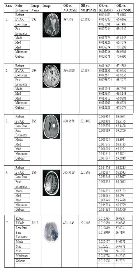
Table 1. Comparison of All the Filters Showing MSE and PSNR of OR. Vs. Noisy Image and OR. Vs. Restored Image

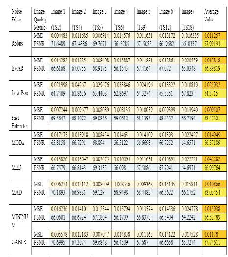
Table 2. Filters Performance Report with their Average MSE and Average PSNR Values

Figure 4 represents the Mean Square Error values for seven different denoised medical images when applied with nine different filters. In this figure, the horizontal axis represents seven different Images with a scale of 1 to 7, while vertical axis represents MSE values. The large value of MSE means that the image is of poor quality.

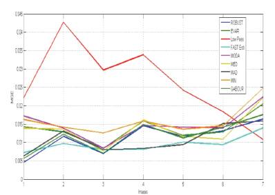
Figure 4. Graph Showing Mean Square Error (MSE) values for 256 × 256 Denoised 7 CT images When Applied with Different Filters

From this Figure, it is clearly depicted that Fast Estimator is best performing followed by Robust filter and Low Pass filter, which is least performing among all filters, except for image number 7, where it performs the best.

Figure 5 represents the Peak Signal to Noise Ratio values for seven different denoised medical images when applied with nine different filters. In this figure, the horizontal axis represents seven different Images with a scale of 1 to 7, while vertical axis represents the PSNR values. A high quality image has higher value of Peak Signal to Noise Ratio.

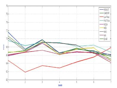
Figure 5. Graph Showing Peak Signal to Noise Ratio (PSNR) values for 256 × 256 Denoised 7 CT images When Applied with Different Filters

6.1 Best Performing Filter

From Table 1 and Figures 4 and 5, it is clear that for Images TS2 and TS5, Robust filter performs best in terms of MSE and PSNR. For Images TS4, Ts6, and TS12, Fast Estimator performs the best. For image TS9, MAD filter performs best, and for Image TS18, Low Pass filter performs best. Hence, we can conclude that, the Fast Estimator performs best with a total count of 3, which is best followed by Robust filter with a total count equal to 2. Then, MAD and Low Pass filter has a count of 1, best with the given set of images.

6.2 Least Performing Filter

From Table 1, and Figures 4 and 5, it is clear that, for Image TS18, Minimum Filter is least performing while for rest of all the images say, TS2,TS4, TS5,TS6,TS9,TS12, Low Pass filter performs least in terms of MSE and PSNR. Hence, we can conclude that, Low Pass filter is the least performing filter among all the filters and with a given set of images.

6.3 Performance Report Based on Average Value of MSE and PSNR

To clarify and to have a better insight in the performance of different filters such as Robust, Evar, Low Pass, Fast Estimator, Moda, Med, MAP, Minimum and Gabor filters the comparison Table 2 is shown.

This Table depicts an average value of MSE and PSNR which is computed from all the given seven images and individual performance of each filter is analyzed with these average values. Therefore, it can be conveniently concluded that, Fast Estimator performs best with these given set of images. The second best filter is MAD followed by Robust as third best filter and Gabor bags the fourth position. Median is fifth, Evar is sixth, Moda is seventh, eighth is Minimum and Low Pass filter comes in ninth position i.e. last in this result.

This paper puts forward an image denoising algorithm based on different noise estimators using Curvelet Transform. To overcome the disadvantages of the wavelet transform along the curves in the images, the Curvelet Transform is used. A new method of application of various noise estimators based on Curvelet transform is used to remove noise from the image. The comparison and performance of different noise estimators is evaluated using Mean Square Error (MSE) and Peak Signal to-Noise Ratio (PSNR) as shown in Figures 4 and 5.The average value of MSE and PSNR of all the images are taken and shown in table 2 as a performance report. From Table 2, it is evident that, Fast Estimator performs better as it gets the highest average value of PSNR, while Low Pass filter is the least performing among the given set of filters. So, the image we obtain by this method is better than that of the traditional wavelet methods.

The authors are very much grateful to the Department of CSE, SSTC, SSGI, FET for giving an opportunity to work on Medical Image Denoising with Various Noise Estimators using Curvelet. They sincerely express their gratitude to Ms. Samta Gajbhiye, Head of Department of computer science and Engineering for giving constant inspiration for this work. They are really thankful to all their friends for their blessing and support.

References

[1]. P. Gravel, G. Beaudoin, and J. A. De Guise, (2004). “A method for modeling noise in medical images”. IEEE Trans. Med. Image., Vol. 23, No. 10, pp. 1221–1232.
[2]. C. J. Garvey and R. Hanlon, (2002). “Computed tomography in clinical practice”. BMJ, Vol. 324, No. 7345, pp. 1077–1080.
[3]. R. Sivakumar, (2007). “Denoising of Computer Tomography Images using Curvelet Transform”. ARPN Journal of Engineering and Applied Sciences, Vol.2, No.1, pp.21-26.
[4]. R. C. Gonzalez and R.E. Woods, (2008). Digital Image Processing. Upper Saddle River, NJ: Pearson Prentice Hall.
[5]. Fodor, I. K. and C. Kamath, (2003). “Denoising through Wavelet Shrinkage: An Empirical Study”. SPIE Journal on Electronic Imaging, Vol. 12(1), pp.151-160.
[6]. Malfait, M. and Roose D., (1997). “Wavelet- based image denoising using a Markov random field a prior model”. IEEE Transactions on Image Processing, Vol. 6(4), pp.549-565.
[7]. Starck J. L., Candes E. and Donoho D. L., (2002). “The Cur velet Transform for Image Denoising". IEEE Transactions on Image Processing, Vol. 11(6), pp.670- 684.
[8]. Starck J.L., Candes E., Murtagh F. and Donoho D.L., (2003). “Gray and Color Image Contrast Enhancement by the Curvelet Transform”. IEEE Transaction on Image Processing, Vol. 12(6), pp.706-717.
[9]. Starck J. L., Candès E. J. and Donoho D. L. (2002). “The Curvelet Transform for Image Denoising”. IEEE Transactions on Image Processing, Vol. 11(6), pp.670- 684.
[10]. Candes E. J., Demanet L., Donoho D. L. and Lexing Ying, (2005). “Fast Discrete Curvelet Transforms”. Stanford University Press Notes.
[11]. Donoho D. L. and Duncan M. R., (2000). “Digital Curvelet Transform Strategy, Implementation and Experiments”. Proc. SPIE, Vol. 4056, pp. 12–29.
[12]. Nguyen Thanh Binh and Ashish Khare, (2010). “Multilevel Threshold Based Image Denoising in Curvelet Domain”. Journal of Computer Science and Technology, Vol.25, pp.632-640.
[13]. Tanjeet Kaur, Gaurav Gupta, Gagandeep Kaur, (2012). “Denoising Of Computed Tomography Images Using Improved Curvelet Transformation”. International Journal of Research in IT & Management, Vol.2 No.7, pp.34-39
[14]. G. Mamatha, L. Gayatri, (2012). “An Image Fusion Using Wavelet And Curvelet Transforms”. Global Journal of Advanced Engineering Technologies, Vol.1, No.2, pp.69- 73.
[15]. Sweta Mehta, Bijith Marakarkandy, (2013). “CT and MRI Image Fusion Using Curvelet Transform“. Journal of information, knowledge and research in Electronics and communication engineering, Vol.2, No.2, pp.848-852.