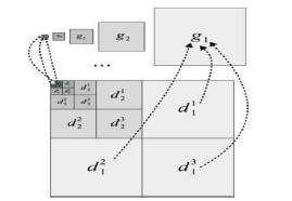
Figure 1. Illustration of Five-Level Gradient Field, Obtained from Five-Level Wavelet Decomposition
Digital watermarking is the act of hiding a message related to a digital signal (i.e. an image, song, video) within the signal itself. In recent years, the phenomenal growth of the internet has highlighted the need for a mechanism to protect ownership of digital media. Digital watermarking is a solution to the problem of copyright protection and authentication of multimedia data while working in a networked environment. The authors propose a robust quantization-based image watermarking method, called the Gradient Direction Water Marking (GDWM), and based on the uniform quantization of the direction of gradient vectors. In GDWM, the watermark bits are embedded by quantizing the angles of significant gradient vectors at multiple wavelet scales. The proposed method has the following advantages: 1) Increased invisibility of the embedded watermark, 2) Robustness to amplitude scaling attacks, and 3) Increased watermarking capacity. To quantize the gradient direction, the DWT coefficients are modified based on the derived relationship between the changes in coefficients and the change in the gradient direction. In this paper, they propose four different denoising techniques for checking of the watermarking efficiency [15]. In various noise scenarios, the performance of the proposed denoised methods are compared in terms of PSNR and Correlation Coefficient. The Contourlet transform provides better PSNR when compared to other filter methods. The Correlation Coefficient observed that the Contourlet transform provides almost near to 1 which is ideal.
In general, any watermarking system that spreads the host signal over a wide frequency band can be called spread spectrum watermarking. In most SS type methods, a pseudo-random noise-like watermark is added (or multiplied) to the host feature sequence. While SS watermarking methods are robust to many types of attacks, they suffer from the host interference problem [1] . This is because the host signal itself acts as a source of interference when extracting the watermark, and this may reduce the detector's performance. To overcome the host interference problem, the quantization (random-binning like) watermarking methods have been proposed. Chen and Wornell (Chen & Wornell, 2001) introduced Quantization Index Modulation (QIM) as a computationally efficient class of data hiding codes which uses the host signal state information to embed the watermark [3]. In the QIM-based watermarking methods, a set of features extracted from the host signal are quantized so that each watermark bit is represented by a quantized feature value. Kundur and Hatzinakos proposed a fragile watermarking approach for the DWT coefficients [2]. Chen and Wornell [3] introduced tamper proofing, where the watermark is embedded by quantizing Quantization Index Modulation (QIM) as a class of data-hiding codes, which yields larger watermarking capacity than SS-based methods. Gonzalez and Balado proposed a quantized projection method that combines QIM and SS [4].
Chen and Lin [5] embedded the watermark by modulating the mean of a set of wavelet coefficients. Wang and Lin embedded the watermark by quantizing the super trees in the wavelet domain [6]. Bao and Ma proposed a watermarking method by quantizing the singular values of the wavelet coefficients [7]. Kalantari and Ahadi proposed a Logarithmic Quantization Index Modulation (LQIM) [9] that leads to more robust and less perceptible watermarks than the conventional QIM. Recently, a QIM-based method, that employs quad-tree decomposition to find the visually significant image regions, has been proposed. Quantization-based watermarking methods are fragile to amplitude scaling attacks. Such attacks do not usually degrade the quality of the attacked media, but may severely increase the Bit-Error Rate (BER). Ourique et al. proposed angle QIM (AQIM), where only the angle of a vector of image features is quantized [8]. Embedding the watermark in the vector's angle makes the watermark robust to changes in the vector magnitude, such as amplitude scaling attacks [15].
One promising feature for embedding the watermark using AQIM is the angle of the gradient vectors with large magnitudes, referred to as significant gradient vectors. This research work proposes an image embedding scheme that embeds the watermark using uniform quantization of the direction of the significant gradient vectors obtained at multiple wavelet scales. The proposed watermarking has several advantages:
Traditional redundant multistage gradient estimators, such as the multi scale Sobel estimator, have the problem of inter scale dependency. To avoid this problem, DWT is employed to estimate the gradient vectors at different scales. To quantize the gradient direction, the Absolute Angle Quantization Index Modulation (AAQIM) is proposed. AAQIM solves the problem of angle discontinuity at θ = π by quantizing the absolute angle value. To quantize the gradient angle, the relationship between the gradient angle and the DWT coefficients is derived. Thus, to embed the watermark bits, the gradient field that corresponds to each wavelet scale is obtained. This is illustrated in Figure 1 [15].
Figure 1. Illustration of Five-Level Gradient Field, Obtained from Five-Level Wavelet Decomposition
Each gradient vector gj corresponds to the three wavelet coefficients dj1 , dj2 , and dj3 . The straightforward way to embed the watermark bits is to partition the gradient fields into non-overlapping blocks. Uniform vector scrambling increases the gradient magnitude entropy, and thus reduces the probability of finding two vectors with similar magnitudes in each block Image. Angle Quantization Index Modulation is an extension of the Quantization Index Modulation (QIM). AQIM has angle discontinuity problem. To solve this problem instead of quantizing the angle, its absolute value is quantized in the interval [θ] Є [0,π].
The quantization function, Q(θ) maps a real angle θ to a binary number as follows:
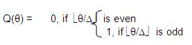
Where, the positive real number Δ represents the angular quantization step size, and  denotes the floor function. The following rules are used to embed a watermark into an angle θ.
Where, w denotes the watermark bit to be embedded.
Cox, I.J. et al. [1] proposed secure spread spectrum watermarking for multimedia, where the embedding capacity is very less. Chen and Wornell [3] introduced tamper proofing, where the watermark is embedded by quantizing Quantization Index Modulation(QIM) as a class of data-hiding codes, which yields larger watermarking capacity than SS-based methods, but Fragile to amplitude scaling attacks, therefore Increased Bit-Error Rate (BER). Ourique, et al. proposed Angle QIM (AQIM), where only the angle of a vector of image features is quantized [8]. Embedding the watermark in the vector's angle makes the watermark robust to changes in the vector magnitude, such as amplitude scaling attacks, but there is Angle discontinuity at θ = π. Kalantari and Ahadi proposed a Logarithmic Quantization Index Modulation (LQIM) [9] that leads to more robust and less perceptible watermarks than the conventional QIM. All these limitations are eliminated by using uniform quantization of the direction of the significant gradient vectors obtained at multiple wavelet scales.
Figure 2 shows the block diagram of the proposed watermark embedding scheme. The watermark is embedded by changing the value of the angle (the direction) of the gradient vectors [11].
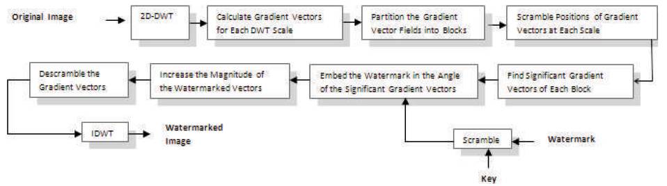
Figure 2. Block Diagram of the Proposed Watermark Embedding Scheme
The embedding process is explained by the following steps:
The watermark bits are decoded following the reverse encoding steps as shown in Figure 3. At the transmitter side, each watermark bit is embedded into the most significant gradient vectors of each block. At the receiver side, they decode the watermark bit of the most significant vectors and assign weights to the decoded watermark bits based on the following rules:
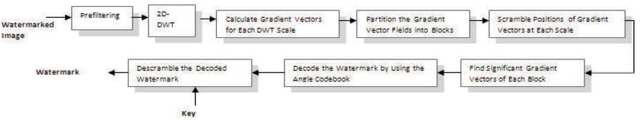
Figure 3. Block Diagram of the Proposed Watermark Decoding Method
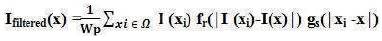
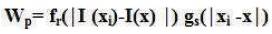
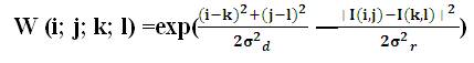
A 512 x 512 Lena as the gray scale original host image and boat as watermark image with size 64 x 64 is shown in Figures 4 (a) and (b) respectively. The watermark is embedded by changing the value of the angle (the direction) of the gradient vectors. First, the 2-D DWT is applied to the host image. At each scale, the gradient vectors are obtained in terms of the horizontal, vertical, and diagonal wavelet coefficients. To embed the watermark, the values of the DWT coefficients that correspond to the angles of the significant gradient vectors are changed. The watermark can be embedded in the gradient direction. The watermarked image and Extracted Watermark is shown in Figures 4 (c) and (d) respectively.
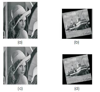
Figure 4 (a) Original Image, (b) Watermark, (c) Watermarked Image (d) Extracted Watermark
Image denoising is an important image processing task, both as a process itself, and as a component in other processes. A number of noise reduction techniques have been developed for images in order to remove noise and retaining edge details. This noise gets introduced during acquisition, transmission & reception and storage & retrieval processes.
The target of de-noising is to purge the noise from an image while maintaining as much as possible the important signal features. There are many ways to denoise an image or a set of data. A good image denoising model's property is that, it will purge noise while preserving edges. Image denoising plays a crucial job in a wide range of applications such as image restoration, visual tracking, image registration, image segmentation, and image classification, where acquiring the original image content is important for robust performance.
Image denoising is an important pre-processing task before further processing of image like segmentation, feature extraction, texture analysis, etc. Due to some different inside (i.e., sensor) and outside (i.e., environment) conditions which cannot be kept away from some practical situations, the noise in images may arise. As a result, there is a degradation in visual quality of an image. So for removing these noises, image denoising algorithms are used. Ideally, the resulting denoised image will not contain any noise or added artifacts. They can say that image denoising is one of the fundamental challenges in the field of image processing, where the underlying goal is to suppress the noise of a contaminated version of an image to estimate the original image. Denoising method is problem specific, because it is based upon the type of image and noise model. The problem of image denoising still remains as an open challenge, especially in situations where the images are acquired under poor conditions and where the noise level is very high. To make the current state-of-art better, researchers keep an attention with it.
A Bilateral filter is a non-linear, edge-preserving and noise reducing smoothing filter for images. The intensity value at each pixel in an image is replaced by a weighted average of intensity values from nearby pixels [12] . This weight is based on a Gaussian distribution. Crucially, the weights depend not only on Euclidean distance of pixels, but also on the radiometric differences (e.g. range differences, such as color intensity, depth distance, etc.). This preserves sharp edges by systematically looping through each pixel and adjusting weights to the adjacent pixels accordingly.
Bilateral filter is first presented by Tomasi and Manduchi in 1998. The concept of the bilateral filter was also presented in as the SUSAN filter and in as the neighborhood filter in different earlier methods. It is mentionable that the Beltrami flow algorithm is considered as the theoretical origin of the bilateral filter, which produces a spectrum of image enhancing algorithms ranging from the 2 L linear diffusion to the 1 L non-linear flows. The bilateral filter takes a weighted sum of the pixels in a local neighborhood; the weights depend on both the spatial distance and the intensity distance. In this way, edges are preserved well while noise is averaged out. Mathematically, at a pixel location x, the output of a bilateral filter is calculated as follows,
where the normalization term Wp , is given as,
As mentioned above, the weight W is assigned using the p spatial closeness and the intensity difference. Consider a pixel located at (i; j) which needs to be denoised in image using its neighboring pixels and one of its neighboring pixels is located at (k; l). Then, the weight assigned for pixel (k; l) to denoise the pixel (i; j) is given by:
where, σd and σᵣ are smoothing parameters and I(i, j) and I(k, l) are the intensity of pixels (i; j) and (k; l) respectively.
After calculating the weights, normalize them,
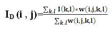
where, ID is the denoised intensity of pixel (i, j).
There are two parameters that control the behaviour of the bilateral filter. σd and σr characterize the spatial and intensity domain behaviours, respectively. In case of image denoising applications, the question of selecting optimal parameter values has not been answered from a theoretical perspective; to the best of our knowledge, there is no empirical study on this issue either.
The edge-preserving de-noising bilateral filter adopts a low pass Gaussian filter for both the domain filter and the range filter. The domain low-pass Gaussian filter gives higher weight to pixels that are spatially close to the center pixel. The range low pass Gaussian filter gives higher weight to pixels that are similar to the center pixel in gray value. Combining the range filter and the domain filter, a bilateral filter at an edge pixel becomes an elongated Gaussian filter that is oriented along the edge. This ensures that averaging is done mostly along the edge and is greatly reduced in the gradient direction. This is the reason why the bilateral filter can smooth the noise while preserving edge structures. On the other hand, the bilateral filter is essentially a smoothing filter. It does not sharpen edges.
Its formulation is simple: each pixel is replaced by a weighted average of its neighbours. This aspect is important because it makes it easy to acquire intuition about its behaviour, to adapt it to application-specific requirements, and to implement it.
The limitations of the bilateral filter are eliminated by using Guided Image Filter (GIF).
A general linear translation-variant filtering process is defined, which involves a guidance image I, a filtering input image p, and an output image q. Both I and p are given beforehand according to the application, and they can be identical [13].
The filtering output at a pixel i is expressed as a weighted average:

where i and j are pixel indexes. The filter kernel Wij is a function of the guidance image I and independent of p. This filter is linear with respect to p.
The key assumption of the guided filter is a local linear model between the guidance I and the filtering output q.
Assume that q is a linear transform of I in a window WK centered at the pixel k.
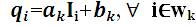
where, (ak , bk ) are some linear coefficients assumed to be constant in wk . A square window of a radius r is used. This local linear model ensures that q has an edge only if I has an edge, because div(q)=a div(I). This model has been proven useful in image super-resolution, image matting, and dehazing.
The comparison of the filtering process using bilateral filter and guided image filter is shown in Figure 5. The bilateral filter requires the kernel size and the intensity range, but using GIF regardless of the kernel size and the intensity range the filtering process can be done.
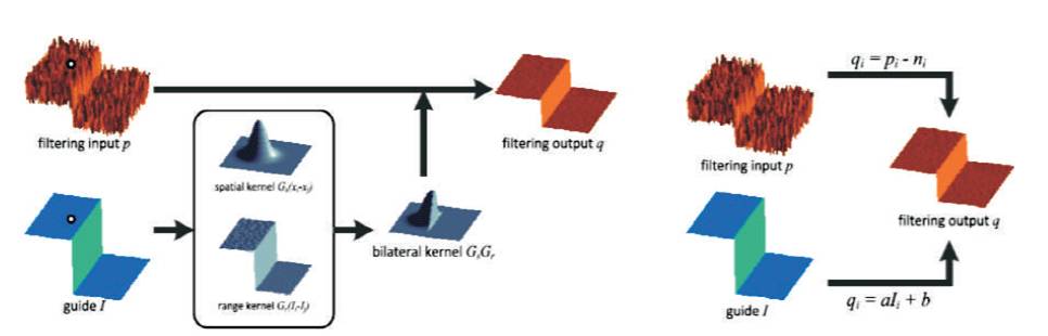
Figure 5. Illustration of the Bilateral Filtering Process (left) and the Guided Filtering Process (right)
To determine the linear coefficients (ak , bk ), using
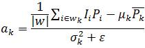
Here, µk and σ2k are the mean and variance of I in wk , |w| is the number of pixels in wk , and  is the mean of p in wk having obtained the linear coefficients (ak , bk ),
The filtering output,  .
.
The guided image filter (Figure 6) has good edge preserving smoothing properties like the bilateral filter, but it does not suffer from the gradient reversal artifacts. The guided filter can be used beyond smoothing. With the help of the guidance image, it can make the filtering output more structured and less smoothed than the input. The guided filter naturally has an O(N) time (in the number of pixels N), non approximate algorithm for both grayscale and high dimensional images, regardless of the kernel size and the intensity range. This is one of the fastest edge preserving filters.
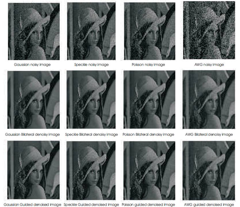
Figure 6. Simulation Results of Watermark Size 64*64
The experimental results are simulated using MATLAB. A 512 x 512 Lena as gray scale original host image and Boat as watermarked image is shown in Figures 4(a) and (b) respectively. Different noise are added to watermark image like Gaussian, speckle, poisson and AWGN. The Simulation results are shown in Figure 6.
The transform of a signal is just another form of representing the signal. It does not change the information content present in the signal. The Wavelet Transform provides a time-frequency representation of the signal. It was developed to overcome the short coming of the Short Time Fourier Transform (STFT), which can also be used to analyze non-stationary signals. While STFT gives a constant resolution at all frequencies, the Wavelet Transform uses multi-resolution technique by which different frequencies are analyzed with different resolutions.
The Wavelet Series is just a sampled version of CWT and its computation may consume significant amount of time and resources, depending on the resolution required. The Discrete Wavelet Transform (DWT), which is based on sub band coding is found to yield a fast computation of Wavelet Transform. It is easy to implement and reduces the computation time and resources required.
The foundations of DWT goes back to 1976 when techniques to decompose discrete time signals were devised. Similar work was done in speech signal coding which was named as sub-band coding. In 1983, a technique similar to sub-band coding was developed which was named pyramidal coding. Later many improvements were made to these coding schemes which resulted in efficient multi-resolution analysis schemes.
In CWT, the signals are analyzed using a set of basis functions which relate to each other by simple scaling and translation. In the case of DWT, a time-scale representation of the digital signal is obtained using digital filtering techniques. The signal to be analyzed is passed through filters with different cut off frequencies at different scales. Wavelet analysis consists of decomposing a signal or an image into a hierarchical set of approximations and information. The levels in the hierarchy often correspond to those in a dyadic scale. From the signal analyst's point of view, wavelet analysis is a decomposition of the signal on a family of analyzing signals, which is usually an orthogonal function method. From an algorithmic point of view, wavelet analysis offers a harmonious compromise between decomposition and smoothing techniques. Unlike conventional techniques, wavelet decomposition produces a family of hierarchically organized decompositions. The selection of a suitable level for the hierarchy will depend on the signal and experience.
Most of the applications of Wavelet Transform is about image processing such as image compression, edge detection, noise removal, etc. The decomposition can continue until the size of the sub-image is small . By setting some parts of its sub-images, the quantity of information is reduced. In other words, the image is compressed by setting the useless data. Edge detection and noise removal are based on the same idea. To detect the edges of the image, the diagonal sub-images are set to zero to obtain the output image with edges clearly.
Wavelet domain is advantageous because DWT makes the signal energy concentrate in a small number of coefficients, hence, the DWT of a noisy image consists of small number of coefficients having high Signal to Noise Ratio (SNR) while relatively large number of coefficients has a low SNR. After removing the coefficients with low SNR, the image is reconstructed using inverse DWT.
The limitations of commonly used separable extensions of one- dimensional transforms, such as the Fourier and wavelet transforms, in capturing the geometry of image edges are well known. In this paper, pursue a “true” two dimensional transform that can capture the intrinsic geometrical structure is the key in visual information [14]. The main challenge in exploring geometry in images comes from the discrete nature of the data. Specifically, construct a discrete-domain multiresolution and multidirectional expansion using non-separable filter banks, in much the same way that wavelets were derived from filter banks. This construction results in a flexible multiresolution, local, and directional image expansion using contour segments, and thus it is named the Contourlet Transform. The discrete contourlet transform has a fast iterated filter bank algorithm that requires an order N operations for N-pixel images. Furthermore, establishing a precise link between the developed filter bank and the associated continuous domain contourlet expansion via a directional multiresolution analysis framework. Showing that with parabolic scaling and sufficient directional vanishing moments, contourlets achieve the optimal approximation rate for piecewise smooth functions with discontinuities along twice continuously differentiable curves.
The natural images are not simply stacks of 1-D piecewise smooth scan-lines; discontinuity points (i.e. edges) are typically located along smooth curves (i.e. contours) owing to smooth boundaries of physical objects. Thus, natural images contain intrinsic geometrical structures that are key features in visual information. As a result of a separable extension from 1-D bases, wavelets in 2-D are good at isolating the discontinuities at edge points, but will not “see” the smoothness along the contours. In addition, separable wavelets can capture only limited directional information–an important and unique feature of multidimensional signals. These disappointing behaviors indicate that more powerful representations are needed in higher dimensions.
Among these parameters, the first three are successfully provided by separable wavelets, while the last two require new constructions. Moreover, a major challenge in capturing geometry and directionality in images comes from the discrete nature of the data: the input is typically sampled images defined on rectangular grids (Figure 7).
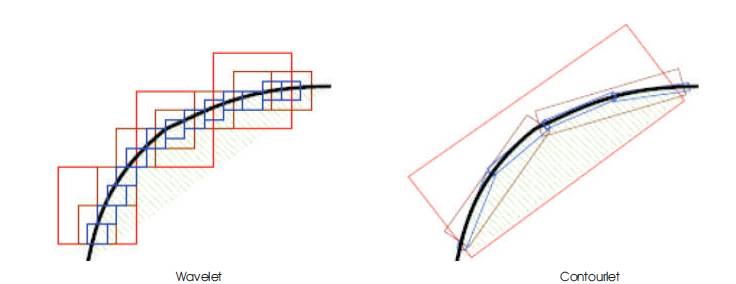
Figure 7. Wavelet Versus Contourlet: Illustrating the Successive Refinement by the Two Systems Near a Smooth Contour
The wavelet is compared with the Contourlet as shown in Figure 8. The improvement of the Contourlet can be attributed to the grouping of nearby wavelet coefficients, since they are locally correlated due to the smoothness of the contours. Therefore, a sparse expansion for natural images is obtained by first applying a multiscale transform, followed by a local directional transform to gather the nearby basis functions at the same scale into linear structures.
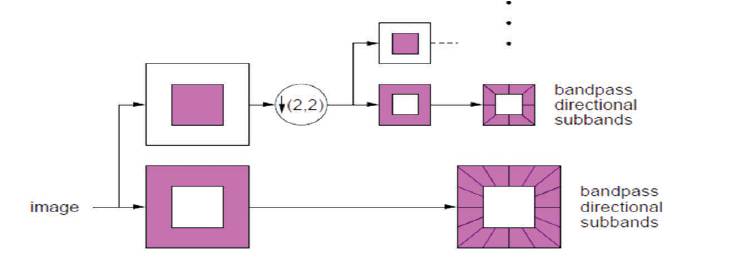
Figure 8. The Contourlet Filter Bank first, a multiscale decomposition into octave bands by the Laplacian pyramid is computed, and then a directional filter bank is applied to each bandpass channel
To construct a multiscale and directional filter bank, the Laplacian Pyramid (LP) is first used to capture the point discontinuities followed by a Directional Filter Bank (DFB) to link point discontinuities into linear structures as shown in Figure 8. The Contourlet Filter Bank explains first, a multiscale decomposition into octave bands by the Laplacian pyramid is computed, and then a directional filter bank is applied to each bandpass channel.
Wavelets are powerful tools in the representation of the signal and are good at detecting point discontinuities. However, they are not effective in representing the geometrical smoothness of the contours. This is because natural images consist of edges that have smooth curves, which cannot be efficiently captured by the wavelet transform. The discrete algorithmic implementation of the curvelet transform poses many problems. The windowing of the sub-band coefficients may lead to blocking effects. To minimize the blocking effect, overlapping windows can be employed, but it will increase the redundancy of the transform. The contourlet transform based on an efficient two-dimensional multi- scale and directional filter bank can deal effectively with images having smooth contours.
The experimental results are simulated using MATLAB. A 512 x 512 Lena as gray scale original host image and Boat as watermarked image as shown in Figures 4(a) and (b) respectively. Different noise are added to watermark image like Gaussian, speckle poisson and AWGN. The Simulation results of watermark size 64*64 is shown in Figure 9.
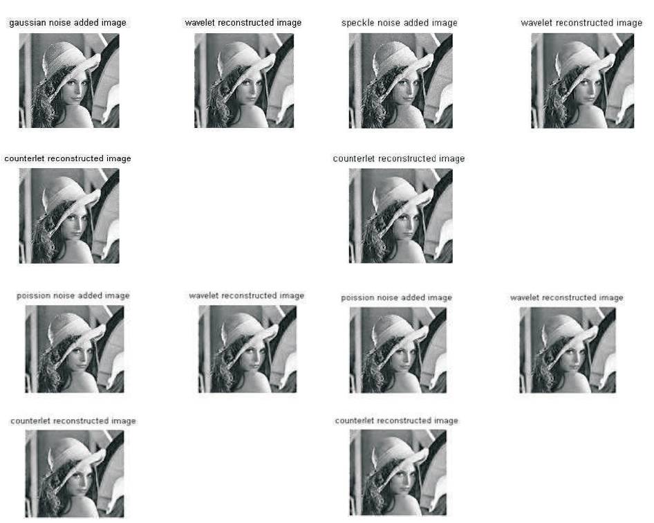
Figure 9. Simulation Results of Watermark Size 64*64
Table 1 and Table 2 presents the comparison of PSNR and Correlation Coefficient of different denoising techniques used for watermarking. From Table 1, it is evident that Contourlet transform provides better PSNR when compared to other filter methods. For example, using Gaussian noise, the PSNR obtained is 127.98 for denoised image. The Correlation Coefficient observed from Table 2 is that Contourlet transform provides almost near to 1 which is ideal.
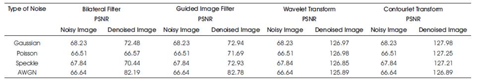
Table 1. Comparison of PSNR of Different Denoising Techniques
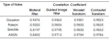
Table 2. Comparison of Correlation Coefficient of Different Denoising Techniques
In GDWM, the watermark bits are embedded by using uniform quantization of the direction of the significant gradient vectors obtained at multiple wavelet scales. The proposed scheme has the following advantages.