Table 1. Prices for Example 1
Companies face a price risk between when they manufacture a product and when the product is made available for selling. Similarly companies also face a price risk from the time lag between purchase of raw materials and its final selling. Hedging (using commodity derivatives) is one of the tools that can be used to minimize the risk arising from price volatility. But hedging in futures is not always a very straight forward process.
The study involves understanding a corporate's requirements – the commodity they are exposed to, their grade / quality, their delivery requirement dates and the type of payout cycle experienced by them. Only then can an appropriate hedging strategy be formulated for them. But even best of hedging solutions can fail if they need to be suddenly squared off due to insufficient MTM funds. Hence when taking a futures position, one needs to get an idea of the approximate maximum MTM margin money that one might be required to pay. VaR margin can be used in this regard.
Most Corporations generally have exposure to fluctuations in various kinds of financial prices, as a byproduct of their operations. Financial prices including foreign exchange rates, interest rates, commodity prices and equity prices all affect a firm's profitability. The effect of these on the reported earnings can at times be overwhelming. Often, you will see firms say in their balance sheets that their income was reduced due to drastic fall in commodity prices or that they enjoyed a huge gain because of strengthening of the Indian Rupees.
Hedging can be one of the methods of reduction in such risks. Broking firms can generate good business if Corporates understand the real benefit of hedging. But hedging is not very generic. Different firms are exposed to different kind of risks, the payout cycle experienced by them vary, so does the commodity required and the side of business-cycle one operates in. This paper explains how broking firms can provide custom-made hedging strategies to the Corporates by understanding their business.
Value At Risk (VaR) can be used to find out what can be the minimum price of a commodity under normal market movements with a certain confidence level. This minimum value can be used to inform a client about the approximate maximum MTM margin requirements on his position. This would be a more explainable and defendable approach for margin calculations than merely taking a certain arbitrary figure.
Also when people invest, they wish to know the amount of risk involved in any particular commodity so that they can choose which commodity to trade in. It's important for a broking house to convey the risk involved, but conveying a theoretical notion of risk to clients may become impossible without some means to quantify risk. VaR is a very important tool in this regard. This paper attempts to implement VaR in Indian commodity market scenario to address both the above issues.
For firms / individual who have an exposure to a particular commodity (either he is a buyer or a producer of it), hedging with futures contracts is one of the most widely used techniques for managing risk. Hedgers who face price uncertainty aim to manage their exposure to adverse movements in spot prices by taking an opposite position in the futures market so that losses in one market is offset by gains in the other. Hedging is not speculation but insurance. The main purpose of hedging is the desire to stabilize income and increase expected profits.
One reason why companies attempt to hedge is because they wish to remove risks that are peripheral to the core business. For example, a electrical copper wire manufacturing firm is known for its quality wires. It's a natural belief that their profits will be driven by the quality of their produce and how well they can market the product and that they apparently do not have exposure to financial/commodity price risk. But that 's a misconception. This company faces a huge amount of price risk due to Copper price variation. Dealing with copper price is not their core business, so they would naturally want to remove any risk arising due to it. Need for hedging is as natural as need for insurance against theft or fire.
Another attraction for hedging the financial price risk of a company, is to improve or maintain its competitiveness. Firms do not exist in isolation. They compete with domestic companies in their sector and with other firms located in foreign countries that produce similar goods. If there are ten companies in a particular sector and seven of them engage in a detailed financial risk management program, then that places substantial pressure on the rest to become more advanced in risk management or face the possibility of being priced out of some important markets. Companies which have proper risk management in place, can use this stability to decrease their cost of procurement or to lower their prices in markets that are deemed to be strategic and essential to the future progress of their firms.
Setting hedging policy is hence a strategic decision. The success or failure this can sometimes make or break a firm. The main issue when choosing a hedging strategy is to strike a balance between uncertainty and the risk of possible opportunity loss. But, hedging is not straight forward thing nor is it a concept that is easy to understand. Hedging objectives vary widely from one to another, even though it appears to be a fairly standard issue, on the face of it. And the spectrum of hedging instruments available is becoming more and more complex every day. Hedging is also dependent on the risk-preferences of the firm's shareholders. There are firms whose shareholders will not take anything under financial price risk while there are other firms whose shareholders might have the capacity to take risk. It is easy to imagine two firms operating in the same sector with similar exposure might have completely different policy, purely because of the differences in their shareholders' attitude towards risk.
But people generally believe investing in futures is only done for trading interest – especially in India commodity hedging is still not used extensively. Futures market is generally considered as a speculative market, but commodities futures market are extremely helpful in hedging also. (Roger W Grey and David J.S. Rutledge). In order to educate people, broking houses themselves need to be able to give correct hedging solutions to business. But different companies have different requirements; their payout cycles vary so does the side of the business cycle they operate in. Hence most corporates require custom – made hedging strategies.
First we need to look into the specific commodity the firm is exposed to. In this regard the easiest thing to do is perfect hedge.
This is the simplest hedging strategy where you simply take an equal and opposite position in the futures market. This is possible only if there is a futures contract that exactly matches, with respect to the nature of the asset and the terms of delivery, the obligation that is being hedged.
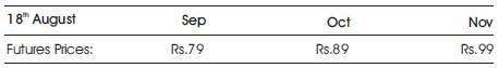
A particular firm requires 5 lots of Aluminium in Sept. i.e. it has to buy 25000 Kg of Aluminium in Sep from the spot market, basis for which will be MCX Price for Sep. On a particular day following (as given in Table 1) are the futures prices:
Procure the commodity from Spot
Take an equivalent position in futures market
He has to bear the Cost of carry
Uncertainty of prices in futures
Table 1. Prices for Example 1
Buys 5 lots (5 x 5000 Kg) of MCX Sep futures @ Rs. 79
Later in September, following (as given in Table 2) are the futures prices:
So, in Futures: It sells 5 lots of MCX Sep futures @ Rs. 89=> Rs.10 'gain'
So, in Spot : Effects purchase of 25000 Kg Aluminium @ 89=> Rs.10 'loss' (Than if he had procured the entire 5Lots on 18th August itself.
Therefore the net effect is: Net of Futures (+Rs.10) and Physical (-Rs.10) = Rs.0
I.e. Has achieved effective Aluminium input price of Rs.79, even though prices rose by Rs.10
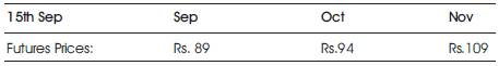
Table 2. Prices for Example 1
On a particular day following (Table 3) are the futures prices:
A particular firm requires 5 lots of Aluminium in Sept. i.e. it has to buy 25000 Kgs of Aluminium in Sep from the spot market, basis for which will be MCX Price for Sep .
Procure the commodity from Spot
Take an equivalent position in futures market
He has to bear the Cost of carry
Uncertainty of prices in futures
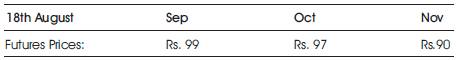
Table 3. Prices for Example 2
Buys 5 lots (5 x 5000 Kg) of MCX Sep futures @ Rs. 99
Later in September, following (as given in Table 4) are the futures prices:
So, in Futures : It sells 5 lots of MCX Sep futures @ Rs.89=> Rs.10 'loss'
So, in Spot : Effects purchase of 25000 Kg Aluminium @ 89=> Rs.10 'profit' (Than if he had procured the entire 5Lots on 18th August itself.
Therefore the net effect is: Net of Futures (-Rs.10) and Physical (+Rs.10) = Rs.0
I.e. Has achieved effective Aluminium input price of Rs.99, even though prices fell by Rs.10
In practice, hedging is often not quite as straightforward. Hence it is not always possible to form a perfect hedge using futures .Some of the reasons is as follows:
Basis = Spot Price – Futures Price of the asset
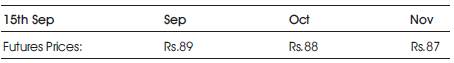
Table 4. Prices for Example 2
Thus in cases mentioned above, need to find way to use sub-optimal contracts, contracts that are highly correlated with the underlying asset and who have a similar variance. One common method of hedging in the presence of basis risk is the minimum variance hedge.
In this we need to find out how many lots of the futures contract one needs to buy of the non similar commodity. In order to get this, the following calculation has to be done :
Notation
Let NA = The number of units of a cash asset needed to be hedged
Let NF = The number of units of the closest futures contract

Let S1 &S2 Be the spot price of the asset in periods 1 & 2
Let F1 &F2 Be the futures price of the closest futures contract in periods 1 & 2.
Let
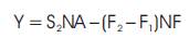
We seek to minimize the variation of Y, which is the difference between the value of the asset at time t = 2, and the value of the futures hedge at time t = 2.
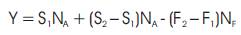
Re- writing (1) we obtain,
Dividing both sides by NA we get,
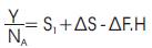
Where ΔS = (S2 –S1 ) and ΔF = (F2 –F1 ) and 
Multiplying both sides by NA we obtain,
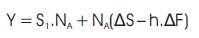
Since S1 and NA are known, the variation in Y depends solely on the variation of 
Statistical aside
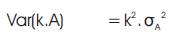
If A and B are random variables, and k is a constant it can be shown that
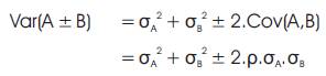
Where ρ is the correlation coefficient between A and B
End of statistical aside
Thus,
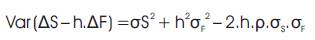
Notice that 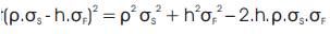
So,
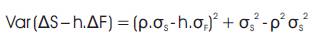
Collecting terms we get,
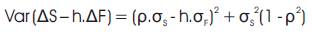
Since  is either positive, or zero (if ρ = 1)
Thus, to minimize Var  , we must minimize ρ.σs -h.σF Or, otherwise stated, to minimize, we set ρ.σs -h.σF = 0 or, ρ.σs = h.σF
then,

Or Hedge Ratio (h) = Correlation (Spot, Futures) * [SD (Spot) / SD (Futures)]
The Hedge ratio (h) above gives number of lots of the futures contract one needs to buy of the non similar commodity in order to hedge.
Hence this hedge ratio is calculated as a first step wherever the commodity requirements of a corporate does not match a standard specifications of any commodity in the futures market.
As a next step, the exact payout cycle of the corporate is analyzed. Also it is ascertained whether he is a buyer of the commodity or a seller i.e. whether he wishes to hedge on the buy side or the sell side.
In order to give a clearer picture, this paper would try to explain hedging strategies with a few of the most commonly occurring business scenarios. Also for anybody who is new to professional hedging solutions, these cases are meant to be a learning tool – a kind of training kit.
(In all these cases its presumed that the initial hedge ratio calculation is done first and then the hedging strategy suggested is followed).
Case 1 : Buyer of Steel
The challenges in this case are the commodity “steel” and the long period of hedge. In India, steel futures have low volumes in far contracts. Hence a long futures position can be taken for current contract only. Before expiry, the position needs to be rolled over to the next contract.
The detailed calculation on the above scenario has been done for the given period Apr 10 to Jan 11 in Table 5.
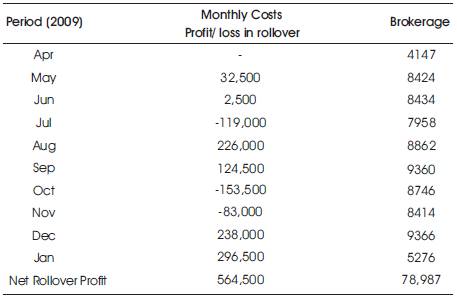
Table 5. Calculation for the Scenario in Case 1
CASE 1: (A Consumer: Buy side Hedge)
In this case the hedging has to ensure that the futures price mirror the kind of average price he achieves in spot only then can the hedge be close to perfect hedge.
With this strategy the prices at which he buys at futures will mirror the kind of prices he achieves using averaging over a month in spot. Hence even in this scenario, he can successfully achieve close to perfect hedge.
A summary of that calculation is given in Table 6. Thus from Table 7 it was found that if the firm had continued to procure copper from the spot only, they would have made a net loss of 43.5 lakhs. But since the futures transaction gives a reverse effect, the losses are mitigated and the net loss figure is only around 6 lakhs.
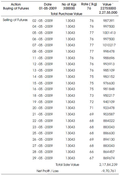
Table 6. Action in Futures Summary Calculation of the Transactions in the Futures Market for the Type 2
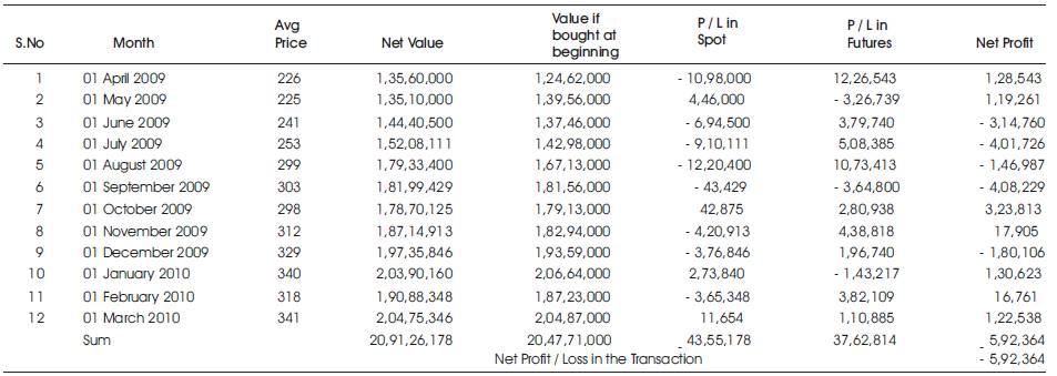
Table 7. Net Effect of Transactions in Futures and Spot Market
As the commodity market evolves in India, the volumes traded increase, and so does the volatility - investors and companies feel the requirement of a risk measurement technique that can be used to limit the risk exposure in commodities. In order to manage risk, first we need to understand “Risk”. Risk is exposure to uncertainty. But risk is a very subjective term. What seems a risky trade to a small investor may be a natural trade for a big corporate client. Also there are many aspects to risk – all of which either an individual is not aware of or may not even understand.
Suppose a CEO wants to know the risk exposure of his firm – the manager knows that there is a certain amount of interest rate risk, market risk, currency risk etc. He can start by listing the company's positions - but this is helpful only if the CEO understands all the positions, the instruments and the risks inherent in them. As such expressing risk to another person becomes very difficult.
Hence, there should be some means to “quantify” risk – one which can be easily understood even by a nonexpert. In this regard “Value At Risk” (VaR) is an important tool. Its simplicity and effectiveness is the reason for its worldwide popularity. According to Glyn A. Holton (1997), around the globe, organizations are racing to implement the new technology.
Value at Risk (abbreviated as VaR) is one of the most popular tools used to estimate exposure to market risks, and it measures the worst expected loss under normal market conditions over a specific time interval at a given confidence level. It was developed in 1993 in response to those famous financial disasters such as Barings's fall.
According to John C Hull (1997), VaR provides a single number to the investors summarizing the total risk in a portfolio of assets “VaR answers the question: how much can I lose with x% probability over a pre-set horizon” (J.P. Morgan, RiskMetrics–Technical Document). Suppose that a portfolio manager has a daily VaR equal to $1 million at 1%. This means that there is only one chance in 100 that a daily loss bigger than $1 million occurs under normal market conditions. With VAR we take the subjective notion risk and describe it in an objective manner.
As with stop loss limits, non specialists intuitively understand the meaning of VAR limits. For e.g. if its stated that 1 day 90% VaR is Rs 1L on an investment in Gold, then the non specialists automatically understands that the investment can lose less than 1L Rs on an average of 9 out of 10 days. The role of the VaR model is to objectively define a range within which a firm's risk should lie – as such it can be used as a “risk measure”.
In general, when N days is the time horizon and X% is the confidence level, VaR is the loss corresponding to the (100 — X) th percentile of the distribution of the change in the value of the portfolio over the next N days as shown in Figure1. For example, when N = 5 and X = 97, it is the third percentile of the distribution of changes in the value of the portfolio over the next five days. Figure above illustrates VaR for the situation where the change in the value of the portfolio is approximately normally distributed. VaR is an attractive measure because it is easy to understand. In essence, it asks the simple question "How bad can things get?" This is the question all senior managers want answered.
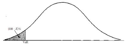
Figure 1. Calculation of Var from the Probability Distribution of Changes in the Commodity Value; Confidence Level Is X%
In theory, VaR has two parameters. These are N, the time horizon measured in days, and X, the confidence interval. In practice, analysts almost invariably set N = 1 in the first instance. This is because there is not enough data to estimate directly the behavior of market variables over periods of time longer than one day. The usual assumption is N-day VaR = 1-day VaR x (N)^0.5. This formula is exactly true when the changes in the value of the commodity on successive days have independent identical normal distributions with mean zero. In other cases it is an approximation.
VaR is not just a number that measures the risk of the firm. VaR can be used to manage risk pro-actively, and firms are finding ways to incorporate VaR to make decisions ranging from capital allocation to setting VaR based trading limits. Some of the uses of VaR are:
There are multiple methods to calculate VaR:
Scenarios used to calculate VAR are drawn from historical market data. For example, the one-day VAR of a portfolio might be estimated with 500 historical scenarios.
A method for calculating VAR for simple portfolios. The closed form model assumes the portfolio's profitability is normally distributed and depends linearly upon applicable risk factors. The portfolios may contain products such as equities, spot, forward or futures, foreign exchange positions, commodities or short-term debt instruments. Closed form VAR will produce erroneous results if applied to portfolios that have significant gamma or convexity, which include portfolios with options, structured notes or mortgage-backed securities.
A methodology for estimating VAR for complex portfolios, which might include options, structured notes or mortgage-backed securities. Scenarios used in calculations are drawn randomly from Monte Carlo simulations.
Delta gamma methodologies abandon the linearity assumption for a parabolic assumption and incorporate second order sensitivities.
All the above methods have some advantages or disadvantages. Historical Simulation is most suited for commodities trading. It is also one of the most widely used measure of VaR . It involves using past data in a very direct way as a guide to what might happen in the future. Suppose that we wish to calculate VaR for a commodity using a one-day time horizon, a 95% confidence level, and 300 days of data.
Procedure to calculate VaR in this method is as below:
The calculations have been done using 300 data points till 30th March, 2010. Data for VaR historical simulation calculation is given in Table 8.
With these we have 300 different scenarios of changes in returns in the commodity. The value of the commodity on the last calculating day (30/3/2010) in the calculation shown) is known. Suppose this is . 351.35. Using this value we can calculate the change in the value of the commodity between 30/3/2010 and 1/4/2010 for all the different 300 scenarios. The calculation is given in Table 9.
The last column in Table 9 shows 300 possibilities for the value of copper on 1/4/2010. These values are then ranked from smallest to largest. The first 15 (= 5% of 300 points) data points correspond to the worst 5% decrease in the value of copper. So the 15th Point 342.18 is the value we are looking for.
Hence it can be said that “We are 95% percent certain that the value of copper might decrease to 342.18 in the next 1 day under normal market conditions by using historical volatility as a risk-metric." Hence a decrease of 9.17 is the VaR.
Similar procedure can be used to calculate VaR of Copper for say 10 day :
N-day VaR = 1-day VaR x (N)^0.5
Therefore 10 day VaR of Copper is = 9.17 x (10)^0.5 = 28.99.
Hence “We are 95% percent certain that the value of copper might decrease to 322 (351.35 – 28.99) in the next 10 days.”
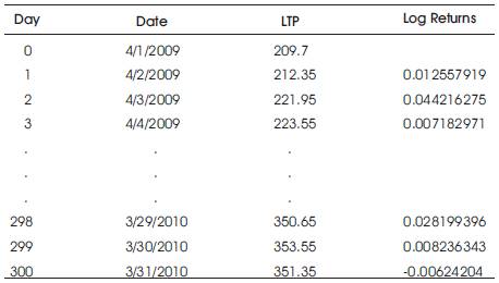
Table 8. Data for VaR Historical Simulation Calculation
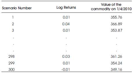
Table 9. 300 Possibilities for the Value of Copper on 1/4/2010
At present if a corporate having a huge investment, wishes to hold on to his position, he has two options:
If a member gets to know the possible minimum values (losses in different positions) for different commodities (with a certain amount of confidence level), they can easily arrive at a definite figure of optimal margin requirements and also be able to justify it.
For calculating margin, MCX and NCDEX use Standard Portfolio Analysis of Risk (SPAN). Standard portfolio analysis of risk (SPAN) is a method used for working out the amount of risk and hence margin required for open short positions in exchange-traded futures. The method was developed by the Chicago Mercantile Exchange and is used widely, for instance, by the London International Financial Futures and Options Exchange. The system uses a scenario building method to work out a range of possible adverse outcomes for futures values against which members have to provide margin. SPAN uses a complex algorithm which takes entire open position (in a single futures class) and treats it as a single portfolio of positions. Factors influencing futures prices such as the price of the underlying, time to expiry, and volatility are used to calculate the possible loss. The method uses historical data to calculate the largest probable one-day change in price: then calculates the effect of a variety of changes in price and volatility on the portfolio. Thus SPAN calculates the potential worst case risk in the portfolio across a number of changes in price and volatility to arrive at the required margin for futures members on a worst case basis.
SPAN generally gives an idea of volatility for only a day – its not very useful if say a position is to be held for 10 days. Also this software is too costly for an average Indian broking house. Rather they can use Value At Risk in this regard.