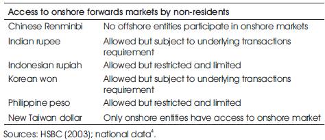
Table 1. Restrictions on various Onshore Markets
The Indian NDF market is less developed as compared to other Asian NDF markets. The Indian NDF market is largely concentrated in Singapore and Hong Kong, with small volumes being traded in the Middle East (Dubai and Bahrain) as well. Some of the foreign banks which trade in the rupee NDF include Deutsche Bank, UBS AG, Standard Chartered Bank, Citibank, JP Morgan Chase, ABN Amro, Barclays 1. Some of the currencies in which NDF is traded are given in the Table 2.
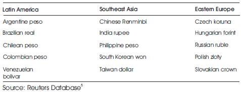
Table 2. Examples of currencies which offer NDF's
Market Turnover
NDF turnover in Indian rupee is seeing a substantial growth in the recent years but still it remains small when compared with onshore market turnover. Moreover the turnover in the Indian rupee NDF market is very small compared to some other Asian currencies traded in the NDF market such as the Korean Won, Chinese Yuan and Taiwanese dollar2 . According to the data given in the Table 3, Korean won is the most liquid market with the highest turnover in NDF market and least bid-ask spread. The transactions in the Indian NDF have also grown significantly over the last few years owing to increased participation by the offshore investors either to hedge or speculate their exposure in the Indian rupee.
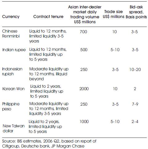
Table 3. Turnover of NDF in Asian Market
1. Literature Review
Park, Jinwoo (2001) observed the interrelation and information flows between the Won–Dollar Spot and NDF markets. Using the augmented GARCH formulation, he found that during the pre-reform period of currency crisis a mean spill over effect existed from the Spot to the NDF market but not vice versa, and volatility spill over effect existed in both directions. After the reform, however, the results were reversed and a mean spill over effect existed from the NDF to the Spot market. Also, the volatility spill over effect existed only in the same direction. Colavecchio Roberta and Funke Michael (2006) 3 used multivariate GARCH techniques to study volatility pullovers between the Chinese Non-Deliverable Forwards market and seven of its Asia-Pacific counterparts over the period January 1998 to March 2005. The empirical results suggested that the Renminbi NDF has been a driver of various Asian currency markets. They found that it was the degree of real and financial integration that exerted the largest influence on volatility transmission. An important study in the area of Indian rupee has been done by Mishra and Behera (2006) 6 where they studied the inter-linkages among the Spot, forwards and NDF markets for Indian rupee. The study found that the NDF market was generally influenced by Spot and forwards markets and the volatility spill over effect existed from Spot and forwards markets to NDF markets. Evidence was also observed for volatility spill over in the reverse direction, i.e., from NDF to Spot market, though the extent was marginal.
Rajesh Chakrabarti (2007) 7 has discussed in detail about the NDF market, its trading volume and reason for its possible growth. He observed that 1-month rupee NDF rates are 50% more volatile than the spot rate and almost 25% more unstable than the onshore forwards rates with volatility rising for long term contacts. The paper also found out that bid-ask spread for Indian NDF is more than those of NDFs in Chinese Yuan and Korean won but lesser than those of Philippine Peso and the Indonesian Rupiah. He also observed that the difference between the onshore forwards rates and NDF rates reflect the effectiveness of capital controls in India. Wang Kai-Li, Fawson Christopher and Chen Mei-Ling (2007) in their research paper found out greater intensity of cross market volatility pullovers in Korea markets, reflecting the considerable information transmitting within Spot, NDF and domestic forwards markets. They further found unidirectional causality of Taiwan Spot to NDF markets. However, the shocks in Taiwan Spot markets were the most influential factor in determining the volatility of NDF and domestic forwards markets.
To measure the effective foreign interest rate (implied NDF yield) Michael Hutchison, Jake Kendall, Gurnain Kaur, Pasricha Nirvikar Singh (2009) in their research paper used the Self Exciting Threshold Auto Regression (SETAR) technique. They found that capital controls have changed over time from primarily restricting outflows to effectively restricting inflows. They also found out that in recent years capital controls have been more symmetric over capital inflows and outflows and the deviations from Covered Interest Parity outside the boundaries are closed more quickly. The most recent work in the context of Indian rupee is done by Anuradha Guru (2009) who observed the interaction and information flow between the INR-Dollar NDF and Spot market, NDF and domestic forwards markets and NDF and exchange traded currency markets over the period 1st January, 2007 to 29th April, 2009. The results indicated that there exists two way causality between returns in Spot and NDF markets and between returns in Deliverable Forwards and NDF market. The test also shows mean and volatility pullovers amongst all the three markets. These results suggest that past returns and innovations in one market exerts influence on the returns in the other market. The paper then looks at the manner, in which these inter-linkages undergo a change post introduction of currency futures on the NSE in September, 2008.
2. Conceptual Framework
2.1 Spread Between Onshore Yields and NDF-implied Yields
An efficient market it is not possible for any trader to earn excess profits as prices reflect all available information. The efficiency/liquidity of the foreign exchange market is 8 often measured in terms of bid/ask spreads 8. More the liquidity, lesser is the spread and vice versa. The spread is almost flat and very low in the Spot segment of the Indian foreign exchange market as a bulk of the transaction is done in this segment of the market. The spread in the NDF segment remains higher than that of the Spot and forwards market reflecting lower liquidity in the NDF market. Moreover due to lesser volume of transaction in the Indian rupee NDFs, the spread remains higher than that of Korean Won.
The forwards exchange rate of the domestic currency is linked to its Spot rate and the interest rate differential between two currencies which is given as:
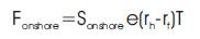
where Fonshore is the forwards rate, Sonshore is the Spot rate, rh is interest rate on the domestic currency and rf is the interest rate on foreign currency, T is the time period for which investment is done. According to interest rate parity theory “currency with lower nominal interest rates should be at a forward premium in terms of currency of the country with the higher interest rates.”
Similarly the NDF market price is linked to onshore spot price by the formula as given:
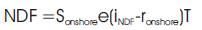
Where iNDF is the NDF-implied offshore interest rate ronshore is the interest prevailing in the onshore market. The arbitrage between the onshore money market and offshore NDF market is ruled out due to restrictions on the offshore participants from entering onshore markets. It is quite possible that iNDF can differ significantly from rh . A large and persistent onshore/offshore spread i.e.(rhonshore -iNDF ) can be attributed to the presence of effective cross-border restrictions. It is this difference which is of great interest to the policy makers as well as the speculators trading in the NDF market.
It is clear from the Figure1 that a one month NDF implied yield is more than domestic. A one month forwards yield for most of the time clearly indicates the effective segmentation of the two markets. It is difficult to compare the onshore and NDF markets as the domestic market is most liquid at short maturities, while NDF markets tend to be more liquid at medium to long maturities9 . The Figure 1 also gives us the clue that there were possibilities of the arbitrage between the onshore currency market and offshore NDF market.
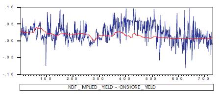
Figure 1. Comparison of NDF Implied Yield and Onshore One Month Forwards Yield 10
2.2 Linkages between Spot, Forwards and NDF Markets for Indian Rupee
There is growing research being done to understand and decipher the linkages between NDF market and domestic Spot and Domestic Forwards (DF) markets for Indian rupee as it is important to know, whether exchange rate in two different markets are at equilibrium or not 11. Any shift from the equilibrium position will lead to arbitrage opportunity. There are various factors contributing to the price mismatch between the two markets. One of the reason as pointed out by Park, Jinwoo (2001) that restrictions on capital account convertibility significantly affect the relation between the offshore NDF and domestic currency markets. The Indian rupee NDF market has developed because of restriction on the capital account convertibility. Thus, knowledge of interrelation and information flows between the offshore NDF and domestic currency markets is important for the investors participating in the two markets. Such an understanding has important implications:
- The stronger correlation between the offshore NDF and domestic currency markets will provide significant inputs to the governments while implementing macroeconomic policies.
- For the hedgers, speculators as well as the arbitrageurs, knowledge of the cross-market relation is important for their investment decisions.
- Interdependence between the offshore NDF and domestic currency markets raises a possibility that one market serves as a primary market for price discovery and the other can take cue from it.
3. Methodology
The data used in the research work consists of daily closing rates of USD/INR Spot, forwards premium/discount and NDF from Reuter's database, Reserve Bank of India. The data period is from 1st January 2007 to 31st March 2010. The methodology used in the paper is divided into two parts:
3.1 Technical Analysis
The study of USD/INR exchange rate primarily through figures for the purpose of analyzing the data which may prove crucial while doing fundamental analysis.
3.2 Fundamental Analysis
Analysis of USD/INR exchange rate using various tools in order to study the trend. Initially Bid-ask spread is calculated to find out the liquidity in the domestic as well as the NDF market. Correlation Analysis is done to find the strength of relation between the onshore spot market and NDF market for different maturities. ARCH and GARCH Model is used to explain the time varying volatility and spillover effect between the given markets. Finally, Granger Causality Test is done to check the direction of causality among different markets.
4. Technical Analysis
4.1 Domestic Forwards Market
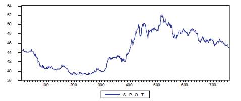
Figure 2. Closing Rates of Domestic Spot for USD-INR12
Figure 2 shows that there is much variation in the USD-INR
exchange rate over the last three years. Before the global
economic slowdown rupee had appreciated to a level of
 `39 against US Dollar. This had exerted a lot of pressure to
the Indian exports business wherein the imports had
become cheaper. The impact of the economic crisis can
be observed from the fact that Indian rupee had depreciated to a level of `52 against US dollar. The Indian
rupee started appreciating again from the fourth quarter
of 2009-2010 which can be attributed to the sound
financial structure of Indian economy.
`39 against US Dollar. This had exerted a lot of pressure to
the Indian exports business wherein the imports had
become cheaper. The impact of the economic crisis can
be observed from the fact that Indian rupee had depreciated to a level of `52 against US dollar. The Indian
rupee started appreciating again from the fourth quarter
of 2009-2010 which can be attributed to the sound
financial structure of Indian economy.
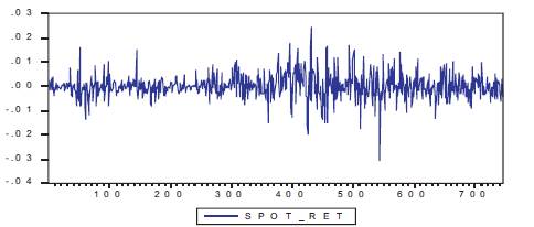
Figure 3. Volatility of Domestic Spot Return for USD-INR13
It is clear from the Figure 3 spot returns, the volatility in the spot market varies between -1% to +1% showing stability in the market. A high spike was seen during the fourth quarter of 2008 when the markets were heavily volatile. The volatility had crossed the normal level indicating confusion in the market during that time. After the financial mess the volatility reduced bringing it back to the normal range.
4.2 Domestic Forwards Market
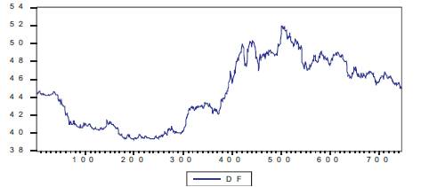
Figure 4. Closing Rates of Domestic One Month Forwards for USD-INR
As evident from Figure 4, it shows a similar characteristics
to the spot market. This is due to the fact that the forwards
rates are quoted based on the interest rate differential
between the two markets so as to avoid any chances of
arbitrage between the two market involved. The rate for
one month forwards depreciated to ` 52 during the
economic slowdown. The forwards rate of Indian rupee
against US Dollar started appreciating which can be
attributed to the investors growing confidence in the
Indian economy. The demand for Indian rupee started
increasing during the fourth quarter of 2008-2009 which resulted in strengthening of Indian rupee.
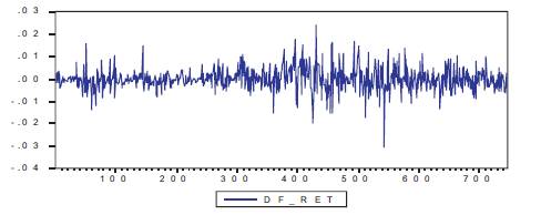
Figure 5. Volatility of Domestic Forwards Return for USD-INR
Figure 5 suggests that the volatility in the domestic forwards market is at the same level as that of spot market. There was a sudden spike in the volatility due to low confidence of the investors during global economic crisis. The spikes were much bigger during the third quarter of 2008-2009. From there it started stabilizing because of the steps taken by the policy makers all across the globe.
4.3 NDF Market (One Month Forwards Rate)
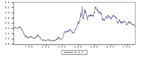
Figure 6. Closing Rates of One Month NDF for USD-INR14
Figure 6 shows the closing rates of one month Rupee Non Deliverable Forwards rate over the period of January 2007 to March 2010 showing more variation than that of one deliverable forwards. This can be attributed to absence of effective controls by policy makers in the NDF market. The NDF market has more spikes than that of the onshore market showing a lesser stability. It can be observed that the NDF rate is usually quoted at higher rate compared to the domestic spot rate. The reason for this can be low liquidity of the market and absence of regulations to some extent. This also gives the arbitragers some chance to get profit
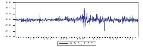
Figure 7. Volatility of One Month NDF Return for USD-INR
Figure 7 shows that the volatility of one month NDF return is in the range of -2 to +2. This suggests that NDF volatility is more than that of one deliverable forwards, showing a greater instability in the NDF market. This can be attributed to lesser liquidity as well as the absence of controls of the policy makers in NDF market.
4.4 Analysis of the Graph of Onshore Spot, Forwards and NDF Market
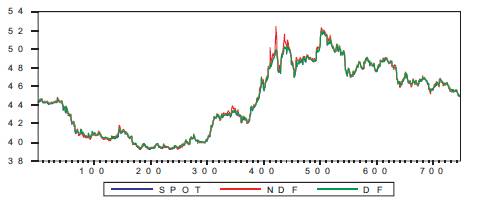
Figure 8. Comparative Analysis of Domestic Spot, Forwards and NDF
Figure 8 gives a better indication of how the domestic markets and NDF market behave. It can be seen clearly that the prices in the NDF market is more than that of corresponding onshore forwards. The difference is more in case of peaks which is due to higher instability of the non deliverable market. The difference in the quote for forwards of different maturity in both the market gives an opportunity to arbitragers to book profits.
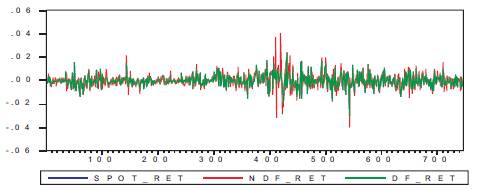
Figure 9. Volatilities of SPOT, Forwards and NDF return for USD-INR
There is more volatility in the NDF market than that of domestic spot as well as forwards market. The findings can be mathematically tested. It is clear from Figure 9 that the global economic slowdown had a major impact in both the NDF market as well as the domestic market. Also, the similarity in the pattern of the returns in both the market indicates the presence of information flow between the two markets.
5. Fundamental Analysis
5.1 Price Discovery
Better the price discovery, lower is the spread. In Table 4 it is clear that the bid-ask spread is more in case of NDF market than that of the domestic market which clearly suggest that the domestic market is more efficient in understanding the price discovery process.
5.2 Liquidity
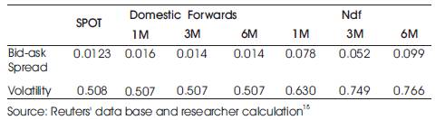
Table 4. Volatility and Bid-Ask Spread In Domestic Spot, Forwards and NDF Market
As observed from the data in Table 4, the spread in domestic market is lower than that of the NDF market of Indian currency, suggesting higher liquidity in the domestic market which is also strongly supported by higher volume of transactions done in the domestic market.
5.3 Volatility
This is one of the most important parameter to observe the stability of any market. Higher the volatility, lower is the stability. From Table 4, we can observe that the volatility in the NDF market is more than that of onshore or domestic forwards market. This is due to the fact that the NDF market is unregulated while the domestic market is governed by Reserve Bank of India.
5.4 Correlation of Domestic Spot with the Forwards in NDF Market
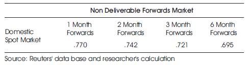
Table 5. Correlation between NDF Market and Onshore Spot Market16
From Table 5, it is clear that the onshore Spot market is strongly correlated to one month forwards NDF market. Moreover it shows a positive correlation among the two markets. From this we can interpret that Spot market serves as the basis for the forwards rate in the NDF market. Another important reason for the positive correlation between the two markets can be attributed to the use of Reserve Bank of India's reference rate (spot rate) to derive the forwards rate of various maturities in the NDF market.
Skewness is a measure of symmetry, or more precisely, the lack of symmetry. The skewness for a normal distribution is zero, and any symmetric data should have skewness near zero. Negative values for the skewness indicate data that are skewed left and positive values for the skewness indicate data that are skewed right17 .
Kurtosis is a measure of whether the data are peaked or flat relative to a normal distribution. That is, data sets with high kurtosis tend to have a distinct peak near the mean, decline rather rapidly, and have heavy tails. Data sets with low kurtosis tend to have a flat top near the mean rather than a sharp peak. A uniform distribution would be the extreme case.
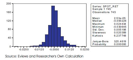
Figure 10. Skewness and Kurtosis of Spot_RET
Clearly we can see from the Figure 10 that SPOT_RET is close to normal distribution with well behaved tails. This is indicated by the skewness of 0.02 and kurtosis of 6.23. A positive value of skewness means that the right tail is longer than that of the left tail.
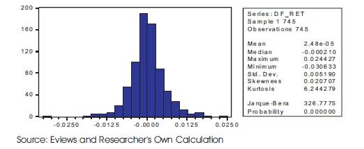
Figure 11. Skewness and Kurtosis of DF_RET
DF_RET shows similar characteristics to that of SPOT_RET. This is indicated by the skewness of 0.021 and a kurtosis of 6.24 as given in the Figure 11. Here also a positive value of skewness shows that the right tail is longer than that of the left tail which is also evident from the diagram. A high value of kurtosis means more of the variance as a result of infrequent extreme deviations.
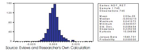
Figure 12. Skewness and Kurtosis of NDF_RET
NDF_RET follows a Cauchy distribution with heavy tails and a single peak at the centre of the distribution. The high value of kurtosis of 10.48 can be explained by the presence of heavy tails as evident from Figure 12. It is comparatively less symmetric than that of the other two as its skewness of 0.225 is much more than that of SPOT_RET and DF_RET. The difference in the value of skewness and kurtosis of NDF_RET can be attributed to more volatility in this market segment.
6. Stochastic Processes
A stochastic process is said to be stationary if its mean and variance are constant over time and the value of covariance between the two time periods depends only on the distance or gap or lag between the two time periods and not the actual time at which the covariance is computed. The general representation of Stationary Stochastic Processes:
Mean: E(Yt )= µ
Variance: Var(Yt )=E(Yt -µ)2 = σ2
Covariance: γt =E[(Yt -µ)(Yt+k - µ)
If a time series is non stationary, we can study its behavior only for the time period under consideration. As a consequence, it is not possible to generalize it to other time periods. Therefore, for the purpose of forecasting, such (non stationary) time series may be of little practical value.
6.1 Tests of Stationarity (The Unit Root Test)
Before we proceed with the data, it is very important to check its stationarity. The starting point of the unit root test is
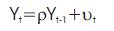
Where νt is a noise error term.
If ρ = 0 then the data is already stationary and the further test can be done on the same data for further analysis. If p =1, then the data is said to be non- stationary and further test is ρ =1 done to make it stationary.
6.1.1 Transforming the Non Stationary Data into Stationary Data
The data are made stationary by taking the first difference which is of the form:

Where Si is the value of the market variable at the end of day i and Si-1 is the value of the market variable at the end of day i-1. The equation also denotes the implied yield of the market. In the research paper SPOT_RET, DF_RET and NDF_RET are implied yield of domestic spot, forwards and non deliverable forwards market. Following are some of the tests to check the stationarity of the data.
6.1.2 Dickey-Fuller (DF) Test
The form for the DF test is

Where t is the time or trend variable. In each case, the null hypothesis is that δ = 0; that is, there is a unit root—the time series is non stationary. The alternative hypothesis is that δ is less than zero; that is, the time series is stationary. If the null hypothesis is rejected, it means that Yt is a stationary time series with zero mean.
6.1.3 The Augmented Dickey–Fuller (ADF) Test
By conducting the DF test it was assumed that the error term νt was uncorrelated. But in νt case are correlated, Dickey and Fuller have developed a test, known as the augmented Dickey–Fuller (ADF) test. This test is conducted by “augmenting” the preceding equation by adding the lagged values of the dependent variable. The ADF test here consists of estimating the following regression:
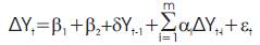
Where εt is a pure white noise error term and where ΔYt-1 = Yt-1 -Yt-2 and so on. The number of lagged difference terms to include is often determined empirically, the idea being to include enough terms so that the error term is serially uncorrelated. In ADF we still test whether δ = 0 and the ADF test follows the same asymptotic distribution as the DF statistic, so the same critical values can be used. One of the major problem in case of ADF test is autocorrelation which is corrected using the Phillips–Perron (PP) Unit Root Tests.
6.1.4 Phillips–Perron (PP) Unit Root Tests
An important assumption of the DF test is that the error terms u are independently and identically distributed. The t ADF test adjusts the DF test to take care of possible serial correlation in the error terms by adding the lagged difference terms of the regressand. Phillips and Perron use nonparametric statistical methods to take care of the serial correlation in the error terms without adding lagged difference terms.
6.1.5 Unit root test results
The testing of unit root properties are done by DF, ADF and PP test. For this analysis the authors have taken six variables as shown in Table 6.The null hypothesis for the test is “the data has a unit root”.
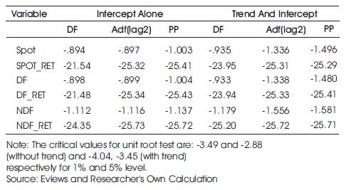
Table 6. The estimated τ statistic values from unit root tests (Level)
Clearly we can observe from Table 6 that the null hypothesis is accepted for variables SPOT, DF, NDF. Thus the data of spot, one month Deliverable Forwards (DF), one month non deliverable forwards are non-stationary at 1% and 5% confidence level. When the unit root test is done on the returns of SPOT, DF, NDF, we can see that tobserved > tcritical for 1% and 5% confidence level. Hence null hypothesis is rejected which means that returns on domestic spot, forwards and NDF are stationary
7. Conceptual Framework
7.1 An Autoregressive (AR) Process
The general representation of AR (p) process is:

Similarly AR (1) is represented as:
where δ is the mean of Y and where νt is an uncorrelated random error term with zero mean and constant variance σ2 (i.e., it is white noise), then we say that yt follows a first- order autoregressive, or AR(1), stochastic process. Here the value of Y at time t depends on its value in the previous time period and a random term; the Y values are expressed as deviations from their mean value.
7.2 Moving Average (MA) Process
Suppose the authors model Y as follows:
where µ is a constant and u, as before, is the white noise stochastic error term. Here Yt at time is equal to a constant plus a moving average of the current and past error terms. Thus, in the present case, we say that Y follows a first-order moving average, or an MA (1), process.
The general representation of MA (q) is:
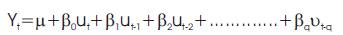
In short, a moving average process is simply a linear combination of white noise error terms.
7.3 Autoregressive and Moving Average (ARMA) Process
It is quite likely that Y has characteristics of both AR and MA and is therefore ARMA. Thus, Yt follows an ARMA (1,1) rocess if it can be written as:
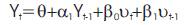
Because there is one autoregressive and one moving average term. Here θ represents a constant term. In general, in an ARMA (p, q) process, there will be p autoregressive and q moving average terms. This is one of the most important step to find out the best fit model for the further analysis of the data.
7.3.1 ARMA Test results
We have taken best fit ARMA model for three variables as shown in Table 7 to rectify the positive autocorrelation that the model was experiencing. Following results were incorporated:
- SPOT_RET follows AR (4) MA (3) model as evident from the p-value given in Table 7. It is clearly shown from the Durbin-Watson Statistics (DW stat) that after incorporating AR (4) MA (3), the DW stat is 1.99 implying almost no autocorrelation.
- DF_RET follows AR (4) MA (4) model. The value of 1.99 for SW stat suggests almost no auto-correlation.
- NDF_RET follows AR (2) MA (2) model with the value of DW stat as 1.98 suggesting negligible auto-correlation.
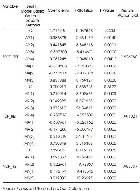
Table 7. Best Fit ARMA Model
7.4 Measuring Volatility in Financial Time Series
Financial time series, such as stock prices, exchange rates, inflation rates, etc. often exhibit the phenomenon of volatility clustering, that is, periods in which their prices show wide swings for an extended time period followed by periods in which there is relative calm.
7.4.1 ARCH- LM Test
This is a Lagrange Multiplier (LM) test for autoregressive conditional heteroskedasticity (ARCH) in the residuals (Engle 1982). The ARCH LM test statistic is computed from an auxiliary test regression. To test the null hypothesis that there is no ARCH up to order q in the residuals, we run the regression
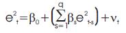
where et is the residual. This is a regression of the squared residuals on constant and lagged squared residuals up to order q.
7.4.2 Arch- Lm Test Results
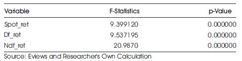
Table 8. Arch- Lm Test
As seen from the findings in Table 8, it has been observed that all the three variables have ARCH effect as suggested by ARCH-LM test. The p-value which is zero in all the three cases suggests the presence of the significant influence of the previous period error terms on the current return distribution. But the structure of volatility will be clearer by GARCH estimation.
7.4.3 Generalized Autoregressive Conditional Heteroskedasticity (GARCH) Test
The most widely used specification is the GARCH (1, 1) model18 introduced by Bollerslev (1986) as a generalization of Engle (1982). Thus, a GARCH (1, 1) model for variance looks like this:
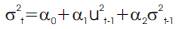
which says that the conditional variance of u at time t depends not only on the squared error term in the previous time period [as in ARCH(1)] but also on its conditional variance in the previous time period. This model can be generalized to a GARCH (p, q) model in which there are p lagged terms of the squared error term and q terms of the lagged conditional variances.
7.4.4 Garch Test Results
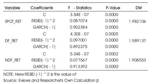
Table 9. Garch Test (VALUE oF α AND β)
Table-9 contains the GARCH (1, 1) estimates with ARCH term represented by RESID (-1) ^2 and GARCH term represented by GARCH (-1). The ARCH and GARCH coefficients are represented as α and β respectively. ARCH component reflects the influence of random deviations in previous period error terms on σ which is a function of random error terms and realized variance of previous periods. Similarly, GARCH coefficient measures the part of the realized variances in the previous period that is carried over in to the current period. The sum of ARCH coefficient and GARCH coefficient (α + β) determines the short run dynamics of the resulting volatility time series. More specifically, a large ARCH error coefficient (α ) means that volatility reacts intensely to market movements and a large GARCH error coefficient (β) indicates that shocks to conditional variance take a long time to die out. So volatility is persistence. If α is relatively high and β is relatively low, then volatility tends to be spikier.
Table 9 suggests that the SPOT_RET, DF_RET and NDF_RET experienced a lower ARCH coefficients (α ) and higher GARCH coefficients (β). It implies that these markets are less sensitive to immediate price movement, but at the same time experiencing a stronger persistence of volatility. Hence current volatility to these market returns can be well analyzed by the help of past return volatility. Also (α + β) <1 in all the three cases which suggests that GARCH (1, 1) model is the best model to explain the volatility in the domestic spot, forwards and non deliverable forwards market.
7.5 The Granger Causality Test
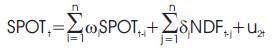
This test is done to find out the direction of flow of information between NDF market and SPOT market, following pair of regression involved:
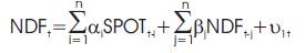
where it is assumed that the disturbances u1t and u2t are uncorrelated.
Following four cases arise:
- Unidirectional causality from SPOT to NDF if
 and
and 
- Unidirectional causality from NDF to SPOT if
 and
and 
- Feedback, or bilateral causality, is suggested when the sets of SPOT and NDF coefficients are statistically significantly different from zero in both regressions.
- Finally, independence is suggested when the sets of SPOT and NDF coefficients are not statistically significant in both the regressions.
7.5.1 Granger Causality Test Results
In order to capture the short term lead lag sensitivity of the domestic spot, forwards and offshore NDF market, the study has used Granger Causality Test for different lag length and the estimated statistics are presented in Table 10. Some of the findings of the test are as follows.
- The null hypothesis of no causality from the SPOT_RET to NDF_RET is rejected at 1% level of probability for different lag length as evident from the p-values given in Table 10.This implies the domestic spot market is significantly causing offshore market. Moreover there is feedback effect from NDF market to domestic spot market showing a bi-directional causality existing between them.
- There exists a bi-directional causality between DF_RET and NDF_RET at 1% probability level. This holds good for all the lag length taken in the paper. It means that there is a two way information flow between these two markets.
- The null hypothesis of no causality is not being rejected for SPOT_RET and DF_RET. This implies a very poor lead lag sensitivity of these two exchange rates with each other.

Table 10. Pair Wise Granger Causality Tests between SPOT_RET, DF_RET and NDF_RET
Conclusion
There exists time varying relation between offshore NDF and domestic spot, forwards market. The results of the paper show the presence of strong GARCH effects with the sum of (statistically significant) estimated coefficients very close to 1, indicating volatility spill over effects between onshore Rupee spot, forwards market and the offshore NDF markets. The result shows bi-directional causality between onshore spot, forwards and NDF market which is in accordance to the various research work done earlier. The paper gives an important result of increasing influence of NDF market on the domestic spot, forwards market. It means that the domestic market takes cue from the information in price changes that originates in the offshore market. Thus, we can say that the NDF market helps in achieving price discovery in the domestic markets. It tells that the policy makers cannot ignore the importance of NDF market in the coming time. Moreover the development of the forwards and futures market in India will also depend on how the NDF market is evolving. NDF market is an intermediate tool which will continue to play an important role till India moves towards fuller capital account convertibility.
Notes
1 http://rbidocs.rbi.org.in/rdocs/Publications/PDFs/80592.pdf
2 http://rbidocs.rbi.org.in/rdocs/Publications/PDFs/80592.pdf
3 http://www.bof.fi/NR/rdonlyres/7FFA4509-D8C6-4D48-9FC0- 73FA75EC92E1/0/dp1606.pdf
6 http://rbidocs.rbi.org.in/rdocs/Publications/PDFs/80592.pdf
7 http://www.isb.edu/media/image/Dec_Insight.p
8 http://www.bis.org/publ/qtrpdf/r_qt0406g.pdf
9 http://rbidocs.rbi.org.in/rdocs/Publications/PDFse/80592.pdf
10 The number on the x-axis of the chart represents 730 data points from 2nd January 2007 to 31st March 2010
11 http://papers.ssrn.com/sol3/papers.cfm?abstract_id=1506710
12 The number on the x-axis of the chart represents 745 data points from 2nd January 2007 to 31st March 2010.
13 The number on the x-axis of the chart represents 730 data points from 2nd January 2007 to 31st March 2010.
14 The number on the x-axis of the chart represents 730 data points from 2nd January 2007 to 31st March 2010
16 The correlation of daily percentage changes of the NDF and onshore Spot rate of Indian rupee against the US dollar of the same tenor. January 2007 to March 2010
17 http://www.itl.nist.gov/div898/handbook/eda/section3/eda35b.htm
18 The (1,1) in parentheses is a standard notation in which the first number refers to how many autoregressive lags appear in the equation, while the second number refers to how many lags are included in the moving average component of a variable