A Study on Granger Causality in the CAPM
Mihir Dash
Head Department of Quantitative Methods, School of Business, Alliance University, Bangalore, India.
Abstract
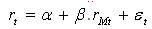
At the heart of the Capital Asset Pricing Model (CAPM) lies the concept of systematic risk. The systematic risk of a security is that component of the total risk of the security that is explained by market risk. This is captured through the regression of security returns rt on market returns rMt , viz
The regression coefficient β(r) measures the sensitivity of returns of the security to changes in market returns.
From an econometric perspective, two concepts become relevant in this context. Firstly, in order for the above regression to be meaningful, the time series {rt} and {rMt} should be stationary. In particular, the presence of a unit root would undermine the significance of β(r), and therefore threaten the entire basis of the CAPM. Secondly, there should be some form of causality from changes in market returns to changes in security returns. In particular, Granger causality from market returns to security returns must hold.
It is in this context that stationarity and Granger causality should be examined for the security line, as represented by the above regression. As Soufian (2001) has pointed out, in order for the regression analyses used for CAPM and APT (Arbitrage Pricing Theory) tests to be meaningful, it is essential to identify the processes that generate the series. In particular, Granger causality may offer an approach to determining the macroeconomic variables that influence asset returns in general.
Keywords :
- Capital Asset Pricing Model,
- Systematic Risk,
- Market Risk,
- Regression,
- Sensitivity,
- Granger Causality,
- Stationarity.
Introduction
The Capital Asset Pricing Model (CAPM), proposed by Treynor (1961), Sharpe (1964), Lintner (1965), and Mossin (1966), is used to determine a theoretically appropriate required rate of return of an asset, given the asset's systematic risk. To do so, the CAPM takes into account the asset's systematic risk, the expected return of the market, and the risk-free rate of return.
The CAPM decomposes an asset's total risk into systematic and specific risk. The systematic risk of an asset is that component of the total risk of the asset that is explained by market risk. This is captured through the regression of asset returns rt on market returns rMt , viz.
Specific risk, or unsystematic risk, is the risk which is unique to each asset. It represents the component of the asset's return which is uncorrelated with general market moves. According to CAPM, the marketplace compensates investors for taking systematic risk, but not for taking specific risk. This is because specific risk can be diversified away. When an investor holds a portfolio, each individual asset in that portfolio entails specific risk, but through diversification, the investor's net exposure is just the systematic risk of the portfolio.
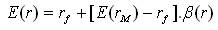
According to the CAPM, the expected return of a portfolio equals the risk-free rate plus the portfolio's beta multiplied by the expected excess return of the market portfolio, i.e.
The security market line, as equation (2) is also called, is the essential conclusion of CAPM. It states that a portfolio's excess expected return over the risk-free rate depends on its beta and not on its volatility; that is, a portfolio's excess return depends upon its systematic risk and not on its total risk.
The CAPM is an asset pricing model because, given a beta and an expected return for an asset, investors will bid its current price up or down, adjusting the expected return so that it satisfies equation (2). Once the expected return is calculated using CAPM, the future cash flows of the asset can be discounted to their present value using this rate to establish the correct price for the asset. In theory, therefore, an asset is correctly priced when its observed price is the same as its value calculated using the CAPM derived discount rate. If the observed price is higher than the valuation, then the asset is overvalued (and undervalued when the observed price is below the CAPM valuation). Alternatively, one can “solve for the discount rate” for the observed price given a particular valuation model and compare that discount rate with the CAPM rate. If the discount rate in the model is lower than the CAPM rate then the asset is overvalued (and undervalued for a too high discount rate). Accordingly, the CAPM predicts the equilibrium price of an asset, assuming that all investors agree on the beta and expected return of any asset. In practice, this assumption is unreasonable, so the CAPM is largely of theoretical value.
The CAPM has several limitations. Firstly, it assumes that asset returns are (jointly) normally distributed random variables. However, it is frequently empirically observed that returns in equity and other markets are not normally distributed; i.e. large swings (often more than three or six standard deviations from the mean) occur in the market more frequently than the normal distribution assumption would expect. It also assumes that the variance of returns is an adequate measurement of risk. This might be justified under the assumption of normally distributed returns, but for general return distributions other risk measures will likely reflect the investors' preferences more adequately. Also, in practice, the CAPM does not appear to adequately explain the variation in stock returns. Empirical studies show that low beta stocks may offer higher returns than the model would predict.
Since beta reflects sensitivity to market risk, the market as a whole, by definition, has a beta of one. Stock market indices are frequently used as local proxies for the market - and in that case (by definition) have a beta of one. An investor in a large, diversified portfolio (such as a mutual fund) therefore expects performance in line with the market. The market portfolio should in theory include all types of assets that are held by anyone as an investment (including works of art, real estate, human capital, and so on), but, in practice, such a market portfolio is unobservable and people usually substitute a stock index as a proxy for the true market portfolio. Unfortunately, it has been shown that this substitution is not innocuous and can lead to false inferences as to the validity of the CAPM, and it has been said that due to the unobservability of the true market portfolio, the CAPM might not be empirically testable.
The Arbitrage Pricing Theory (APT), proposed by Ross (1976, 1977), is a general theory of asset pricing that generalizes the CAPM. The APT holds that the expected return of a financial asset can be modeled as a linear function of various macro-economic factors or theoretical market indices, where sensitivity to changes in each factor is represented by a factor-specific beta coefficient.
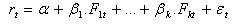
Similarly to the CAPM, the APT decomposes a portfolio's risk into systematic and specific risk. This is captured through the regression of portfolio returns rt on a set of risk factors F1 , … Fk , viz.
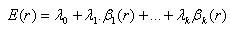
The regression (3), known as the first-pass regression, identifies the portfolio's factor sensitivities β1 , … βk , which, similarly to the CAPM's β(r), measure the sensitivity of the portfolio returns to changes in the risk factors. According to APT, the expected return of a portfolio is linearly related to its factor sensitivities, i.e.
where λ1 , … λk represent risk premia corresponding to each of the risk factors F1 , … Fk . The model in equation (4) is estimated by regression of portfolio returns on the factor sensitivities, yielding estimates for the risk premia.
The APT asserts that equation (4) can be used to find the expected return of a portfolio given its factor sensitivities. The model-derived rate of return will then be used to price the asset correctly - the asset price should equal the expected end of period price discounted at the rate implied by model. If the price diverges, arbitrage should bring it back into line.
The APT describes the mechanism, whereby arbitrage by investors will bring an asset which is mispriced, according to the APT model, back into line with its expected price. Note that under true arbitrage, the investor locks-in a guaranteed payoff, whereas under APT arbitrage as described below, the investor locks-in a positive expected payoff. The APT thus assumes arbitrage in expectations - i.e. that arbitrage by investors will bring asset prices back into line with the returns expected by the model portfolio theory. In the APT context, arbitrage consists of trading in two assets, with at least one being mispriced. The arbitrageur either sells the asset which is relatively overpriced and uses the proceeds to buy one which is correctly priced, or sells an asset that is correctly priced and uses the proceeds to buy the asset that is relatively underpriced. A correctly priced asset in this context may be in fact a synthetic asset - a portfolio consisting of other correctly priced assets - which has the same exposure to each of the macroeconomic factors as the mispriced asset. When the investor is long the asset and short the portfolio (or vice versa), he has created a position which has a positive expected return (the difference between asset return and portfolio return) and which has a net-zero exposure to any macroeconomic factor and is therefore risk free (other than for firm specific risk). The arbitrageur is thus in a position to make a risk-free profit.
The APT differs from the CAPM in that it is less restrictive in its assumptions. It allows for an explanatory (as opposed to statistical) model of asset returns. In some ways, the CAPM can be considered as a special case of the APT, in that the securities market line represents a single-factor model of the asset price, where beta is exposed to changes in value of the market. The APT can be seen as a supply side model, since its beta coefficients reflect the sensitivity of the underlying asset to economic factors. Thus, factor shocks would cause structural changes in the asset's expected return, or in the case of stocks, in the firm's profitability. On the other hand, the CAPM is considered a demand side model. Its results, although similar to those in the APT, arise from a maximization problem of each investor's utility function, and from the resulting market equilibrium (investors are considered to be the consumers of the assets).
As with the CAPM, the factor-specific betas are found via a linear regression of historical security returns on the factor in question. Unlike the CAPM, the APT, however, does not itself reveal the identity of its priced factors - the number and nature of these factors is likely to change over time and between economies. As a result, this issue is essentially empirical in nature. Chen et al. (1986) identified the following macro-economic factors as significant in explaining security returns: surprises in inflation; surprises in GDP as indicted by an industrial production index; and surprises in investor confidence due to changes in default premium in corporate bonds. In practice, indices or spot or futures market prices may be used in place of macro-economic factors, which are reported at low frequency (e.g. monthly) and often with significant estimation errors. Market indices are sometimes derived by means of factor analysis. More direct indices that might be used are: short term interest rates; the difference in long-term and short term interest rates; a diversified stock index; oil prices; gold or other precious metal prices; currency/exchange rates, and other macroeconomic variables.
1. Literature Review
There is abundant empirical evidence indicating that the source of risk introduced in CAPM does not explain the cross-sectional expected returns, such as Fama and French (1995, 1996), suggesting that one or more additional factors may be required to characterize the behavior of expected returns. A number of studies have examined the impact of firm-specific variables such as firm size and book-to-market-value, as in Fama and French (1992), while other studies have examined the impact of the macro-economic factors, as in Chen et al. (1986), Antoniou et al. (1998), and Poon and Taylor (1991).
A major issue in the empirical analysis of any asset pricing model, apart from the question of whether it adequately prices the assets, is that it must be robust enough whilst simultaneously offering economic insight into the determinants of security returns. Fama (1991) argued that a model requires more evidence on how different factors explain pricing assets in different samples. Therefore, to determine the economic factors, influencing pricing is not sufficient to assess the empirical content of APT. The validity of APT also depends on its ability to price assets outside of the sample used for estimation. Fama (1991) argued that the relations between returns and economic factors may be spurious requiring for a robustness check outside the sample studied. Connor and Korajczyk (1992) argued that a testable implication of the APT is the equality of the prices of risk across different sub-samples of assets. Antoniou et al. (1998) examined the uniqueness of the returns generating process for two sub-samples of assets. Using the estimation method that allows idiosyncratic returns to be correlated across assets, they found that three factors are unique in the sense that they carry the same prices of risk in both samples.
Malkamäki (1993) examined the CAPM using timevarying- parameter models. Prior evidence does not support the CAPM in that it suggests that market risk is not priced or that the price of the beta risk is significantly negative for a thin European stock market, e.g. the Finnish stock market. He showed explicitly that this phenomenon is due to static ordinary least squares beta estimates which are spurious, and reduced the errors-in-variables problem by estimating firm-specific betas using Kalman filter techniques and employed the betas forecasted on the basis of these estimated betas in a cross-sectional analysis. Analysis of pooled data showed that the price of conditional risk is positive and that the mean-variance efficiency of the market index cannot be rejected, supporting the CAPM.
Soufian (2001) investigated the validity of CAPM and APT for securities traded on the London Stock Exchange, in order to explain pricing across time, taking three different sub-samples of time periods on the basis that during each subset of samples, the UK economy experienced different economic conditions (1980-1997). Soufian (2001) applied the two-stage procedure analysis of Fama and McBeth (1973) to test the proposition that at any point in time there is a linear and positive relationship between CAPM's β coefficient and expected returns.
Soufian (2001) used time series techniques for the prewhitening process. Before testing the relationship between stock returns and macro-economic series, it is essential to identify the process that is generating the series. If an input series is auto-correlated, the direct crosscorrelation function between the input and response series gives a misleading indication of the relation between the input and response series. Since the estimated risk premia in asset pricing are sensitive to the way that the unexpected components are generated to test the APT and CAPM, it is essential to use an appropriate method to generate the unanticipated factors. Statistically, it is possible to obtain the time series of unexpected movements by identifying and estimating a vector auto-regressive model in an attempt to use its residuals as the unexpected innovations in the economic factor. Soufian performed the pre-whitening process for the input series; market portfolios and the macroeconomic series, by fitting an univariate ARIMA model to each series sufficient to reduce the residuals to white noise, and then filtering the input series with this model to get the white noise residual series.
Davidson et al., (2002) argued that, to the extent that asset pricing models are employed by investors and corporations for decision making purposes, the CAPM is the most likely candidate. As Fama and French (1997) asserted, “the choice of model is important”. Davidson et al., examined whether the CAPM-β is a good proxy for the “true” factors that drive returns, following the work of Born and Moser (1990) and Wei (1988). Born and Moser (1990) calculated factor loadings on six factors (using principal component analysis) for the thirty stocks that comprise the Dow Jones Industrial Index in the period 1962-1982, and regressed the factor loadings against the corresponding β's. They found evidence that β is a “consensus” risk factor: at the 5% significance level they reported that three factors are priced, and at the 10% level an additional factor is priced (Born and Moser, 1990). Davidson followed a similar methodology, using an endogenous APT model where the factors are extracted from the returns data using factor analysis, and found evidence that the international CAPM beta is a consensus measure of up to four return generating factors.
Thus, though several studies address the empirical testing of the CAPM and the APT, very few use time series techniques. As Soufian (2001), has pointed out, in order for the regression analyses used for CAPM and APT tests to be meaningful, it is essential to identify the processes that generate the series. In particular, Granger causality on security returns has not been analyzed in the literature.
The present study examines Granger causality in the context of the CAPM for Indian stocks. Two concepts, in particular, become relevant in this context. Firstly, there should be some form of causality from changes in market returns to changes in security returns. In particular, Granger causality from market returns to security returns must hold. Secondly, in order for the security line to be meaningful, the time series {rt} and {rMt} should be stationary. In particular, the presence of a unit root would undermine the significance of β(r), and therefore threaten the entire basis of the CAPM.
2. Data and Methodology
The objective of the study was to investigate Granger causality between the daily returns of stocks and the daily returns of the stock market index (NIFTY) in the National Stock Exchange (NSE), India. The data for the study consisted of the daily closing prices of a sample of thirty stocks listed on the NSE and the NIFTY over the period of five years, from January 1, 2003 through December 31, 2007. The sample stocks were selected by simple random sampling from the NSE-listed stocks. The data was collected from the NSE website/archives.
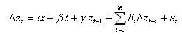
The first step involved the augmented Dickey-Fuller unit root test to test the series for stationarity. The formulation for this test is given by,
where Δzt = zt - zt-1 is the first order forward difference in the time series is {zt}, zt-1 is the one-period lag in the time series {zt} and Δzt-i , and the largest value of Δzt . The coefficient α represents the drift parameter, β represents the trend parameter, and γ represents the unit root. The order m is the optimal lag chosen by Akaike's (1969) information criterion. The augmented Dickey-Fuller test rejects the presence of a unit root if γ is significant and negative.
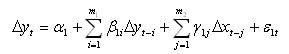
The next step involved the linear Granger causality tests (1969). The Granger causality tests involve the estimation of the following models:
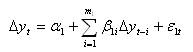
with the restricted model:
with the restricted model:
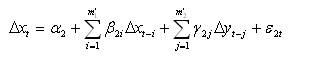
- For testing causality of daily returns of NIFTY on daily returns of the stocks, compare the unrestricted model:
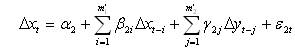
- For testing causality of daily returns of the stocks on daily returns of NIFTY, compare the unrestricted model:
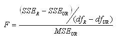
where Δxt = xt - xt-1 is the first order forward difference in the daily returns of NIFTY and Δyt = yt - yt-1 is the first order forward difference in the daily returns of the stocks; α, β, γ are the parameters to be estimated, and ε1 , ε2 are standard random errors with zero mean and constant variance. Finally, the orders m1 , m2 , m1’, m2’ are the optimal lags chosen by Akaike's (1969) information criterion. In order to test the significance of γ1 and γ2, the usual F-statistic as below is employed:
Significance of either of the coefficients γ1 or γ2 indicate Granger causality between changes in daily returns of NIFTY and changes in daily returns of the stocks. If both γ1 and γ2 are statistically significant, then there is bi-directional causality between changes in daily returns of NIFTY and changes in daily returns of the stocks. Finally, if neither of γ1 and γ2 are statistically significant, then no causality exists between daily returns of NIFTY and daily returns of the stocks.
3. Findings
The augmented Dickey-Fuller unit root tests were performed for the selected stock market indices to determine stationarity. The results of the tests are shown in Table 1.
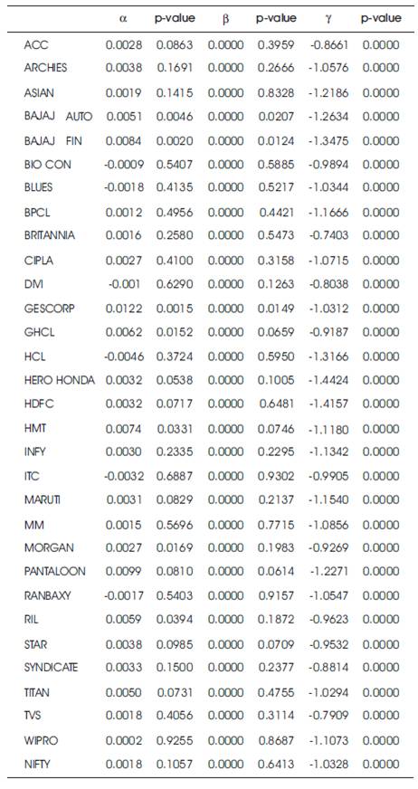
Table 1. Results of Augmented Dickey-Fuller Unit Root Tests
The results of the augmented Dickey-Fuller unit root tests indicate that, for all the daily returns of stocks and the daily returns of NIFTY, the hypothesis of a unit root is rejected. The tests also indicate that, for some of the stocks, there is a significant drift component, and, for some of the stocks, there are significant drift and trend components.
The Granger causality tests were performed to test the direction of causality between the daily returns of stocks and the daily returns of NIFTY. In performing the tests, a lag structure of twenty lags were chosen, as auto correlations in the first order differences in all of the selected stocks and the stock market index NIFTY were significant up to twenty lags. The results of the tests are shown in Table 2.
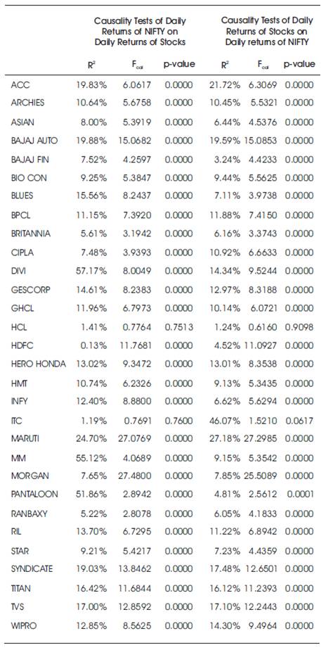
Table 2. Results of Granger Causality Tests
The results of the Granger causality regressions indicate that there was significant bi-directional causality between the daily returns of NIFTY and the daily returns for 93.33% of the sample stocks, while for 6.67% of the sample stocks there is no significant causality in either direction. In particular, with 95% confidence, in at most 14.16% of all NSE-listed stocks can be bi-directional causality of stock daily returns with NIFTY daily returns be expected to fail.
Conclusions
The CAPM and the APT are the two most influential theories on asset pricing. There is abundant empirical evidence indicating that market risk alone does not explain the cross-sectional expected returns, suggesting that one or more additional factors may be required to characterize the behavior of expected returns. A number of studies have examined the impact of firm-specific variables such as firm size and book-to-market-value, while other studies have examined the impact of the macro-economic factors. The present study examines Granger causality in the context of the CAPM for Indian stocks.
The results of the Granger causality regressions indicate that, for 93.33% of the sample stocks, there was significant bi-directional causality between stock returns and market returns, so that the security line, represented by the regression (1) is meaningful for these stocks. On the other hand, for 6.67% of the sample stocks, there was no significant causality of stock returns with market returns in either direction, indicating in particular that market returns did not explain stock returns for these stocks. Thus, overall, it can be concluded that, though market returns is a necessary factor in explaining individual stock returns, it in itself it does not explain stock returns; i.e. it cannot be the only explanatory factor involved. Thus, the security line as represented by the regression equation (1) is inadequate; other factors would need to be introduced in order to explain stock returns more completely. Thus, the results are consistent with the Arbitrage Pricing Theory (APT).
The results of the study suggest that time series techniques play an essential role in the empirical testing of the CAPM and the APT. As Soufian (2001) has pointed out, in order for the regression analyses used for CAPM and APT tests to be meaningful, it is essential to identify the processes that generate the series. In particular, Granger causality may offer an approach to determining the macroeconomic variables that influence asset returns in general.
References
[1]. Akaike, H., (1969). “Fitting autoregressive models for prediction”. Annals of the Institute of Statistical Mathematics, Vol.21, No.1, pp.243-247.
[2]. Antoniou, A., Garrett, I., and Priestely, R., (1998). “Macroeconomic variables as common pervasive risk factors and the empirical content of the arbitrage pricing theory”. Journal of Empirical Finance, Vol.5, No.3, pp.221-240.
[3]. Born, J.A., and Moser, J.T., (1990). “Bank equity returns and changes in the discount rate”. Journal of Financial Services Research, Vol.4, No.3, pp.223-241.
[4]. Chen, N-F, Roll, R., and Ross, R., (1986). “Economic forces and the stock markets”. Journal of Business, Vol.59, No.3, pp.383-403.
[5]. Connor, G., and Korajczyk, R.A., (1992). “The Arbitrage Pricing Theory and Multifactor Models of Asset Returns”. LSE Financial Markets Group Discussion Paper No. 149, London School of Economics.
[6]. Davidson, S., Faff, R., and Mitchell, H., (2002). “Are Returns in the International Economy Explained by a Single or Multi-factor Structure?” Studies in Econometrics and Economics, Vol.26, No.1, pp.17-32.
[7]. Fama, E., (1991). “Efficient Capital Markets: II”. Journal of Finance, Vol.46, No.5, pp.1575-1617.
[8]. Fama, E., and French, K.R., (1992). “The Cross-section of Expected Stock Returns”. Journal of Finance, Vol.47, No.2, pp.131-155.
[9]. Fama, E., and French, K.R., (1995). “Size and Book-to- Market Factors in Earnings and Returns”. Journal of Finance, Vol.50, No.1, pp.427-465.
[10]. Fama, E., and French, K.R., (1996). “The CAPM is Wanted, Dead or Alive”. Journal of Finance, Vol.51, No.5, pp.1947-1958.
[11]. Fama, E., and French, K.R., (1997). “Industry costs of equity”. Journal of Financial Economics, Vol.43, No.2, pp.153-193.
[12]. Fama, E.F., and McBeth, J.D., (1973). “Risk, return, and equilibrium: empirical test”. Journal of Political Economy, Vol.81, No.3, pp.607-636.
[13]. Granger, C.W.J., (1969). “Investigating causal relation by econometric and cross-sectional method”. Econometrica, Vol.37, pp.424-438.
[14]. Lintner, J., (1965). “The Valuation of Risk Assets and the Selection of Risky Investments in Stock Portfolios and Capital Budgets”. The Review of Economics and Statistics, Vol.47, pp.13-37.
[15]. Malkamäki, M., (1993). Essays on Conditional Pricing of Finnish Stocks, Helsinki: Bank of Finland Publications, Series B.
[16]. Mossin, J., (1966). “Equilibrium in a Capital Asset Market”. Econometrica, Vol.34, No.4, pp.768-783.
[17]. Poon, S., and Taylor, S.J., (1991). “Macroeconomic factors and the UK stock market”. Journal of Business Finance and Accounting, Vol.18, No.5, pp.619-636.
[18]. Ross, S., (1976). “The Arbitrage Theory of Capital Asset Pricing”. Journal of Economic Theory, Vol.13, No.3, pp.341-489.
[19]. Ross, S., (1977). “Return, Risk and Arbitrage”. In Risk and Return in Finance. Cambridge, MA: Ballinger.
[20]. Sharpe, W.B. (1964). “Capital Asset Prices: A Theory of Market Equilibrium under Conditions of Risk ”. Management Science, Vol.9, No.2, pp.277-293.
[21]. Soufian, N. (2001). “Empirical Content of Capital Asset Pricing Model (CAPM) and Arbitrage Pricing Theory (APT) Across Time”. Manchester Metropolitan University Business School Working Paper Series, WPS010.
[22]. Treynor, J.L., (1961). “Market Value, Time, and Risk”. Unpublished manuscript “Rough Draft” dated 8/8/61, #95-209.
[23]. Wei, J. (1988). “An Asset Pricing Theory Unifying the CAPM and APT”. The Journal of Finance, Vol.43, No.4, pp.881-892.