Table 1. Relationship Between Sampling Fraction and Fixed Random Factors
Gas Metal Arc Welding (GMAW) has got many wide applications in today's industry. Selection of input welding parameters in this process plays a very major role depending on which the quality of weld and subsequently the productivity depends. Controlling of the input parameters is very much essential to obtain a good quality weld. In the present work some of the parameters such as, welding voltage, welding current, welding speed, Nozzle to Plate Distance (NPD) and Gas Density (G) influencing weld deposit area in Gas Metal Arc welding process are studied by carrying out experimentations and also a mathematical model has been developed for achieving better weld deposit area in a mild steel specimen. Factorial design approach is applied for finding the relationship between the various process parameters and weld deposit area. The study discovered that, the welding voltage and Nozzle to Plate Distance is varying directly with weld deposit area and a direct relationship existing between the welding current and speed with weld deposit area is observed.
Gas Metal Arc Welding (GMAW) is an arc welding process that joins metals. It does this by heating the metals with an electric arc. The arc is between a continuous, consumable electrode wire and the workpiece. The arc is shielded from contaminants in the atmosphere by a shielding gas. GMAW had its beginning in the late 1940's. It was developed to speed up welding that was being done by the Gas Tungsten Arc Welding (GTAW) process. GTAW is also an arc welding process shielded by shielding gas, but GTAW uses a non consumable tungsten electrode. The filler rod for GTAW is generally added manually at a much slower rate. GMAW was thus developed to make welding a faster, more profitable process. GMAW developed when GTAW was thought to be too slow for a process to weld thick sections of aluminum. Whereas GTAW worked very well on thin gauges (literally melting the metals together without adding filler wire), GMAW became much more efficient and profitable for welding thicker materials. This became especially helpful during the years of World War II. During its early days, Gas Metal Arc Welding was generally done with small electrode wires, high heat, and shielding gases that were inert (nonreactive) (Karadeniz et al. 2007). Because an inert gas was used, the term Metal Inert Gas, or 8 MIG welding, was used to refer to this process. This term is still a very common reference for the welding process, even though technically incorrect. The development over the years of the use of reactive shielding gases (Metal Active Gas − MAG welding) (Suban and Tusek, 2003, Quinn et al. 1999) gave rise to the term Gas Metal Arc Welding, or GMAW. Following WW II, the peace time economy saw an increase of the economical Gas Metal Arc Welding process. In addition to being more profitable on heavy aluminum weldments, GMAW was refined to produce quality weldments on other materials and thicknesses, both thin and thick. Thus, the GMAW process unfolded into becoming a major element in industry today.
Gas Metal Arc Welding can be done in basically three different ways. Semiautomatic welding means that the equipment controls only the electrode wire feeding. The movement of the welding gun is controlled by hand. Thus, semiautomatic welding is sometimes called handheld welding. Machine welding uses a gun that is connected to a manipulator of some kind (not handheld). An operator has to constantly set and adjust controls that move the manipulator. (Jang et al. 2005, Praveen and Yarlagadda, 2005a). Automatic welding uses equipment which welds without the constant adjusting of controls by a welder or an operator. On some equipment, automatic sensing devices control the correct gun alignment in a weld joint.
GMAW process overcome the restriction of using small lengths of electrodes and overcome the inability of the submerged-arc process to weld in various positions. By suitable adjusting the process parameters, it is possible to weld joints in the thickness range of 1-13 mm in all welding position (Kuk et al. 2004, Murugan and Parmar, 1994).
All the major commercial metals can be welded by GMAW (MIG/CO ) process, including carbon steels, low alloy and 2 high alloy steels, stainless, aluminum, and copper titanium, zirconium and nickel alloys (Quintino and Allum, 1981, Praveen and Yarlagadda, 2005b).
The short circuit transfer gets its name from the welding wire actually "short circuiting" (touching) the base metal many times per second. When the welding gun trigger is pressed, the electrode wire feeds continuously from the wire feeder, through the gun, and to the arc, short circuiting to the base metal. In the course of welding, this cycle can repeat itself between 20 and as much as 250 times per second. An average welding condition, however, would average between 90 and 150 short circuits per second. The number of short circuits per second will depend upon such things as slope and inductance settings, the size wire that is being used, and the Wire Feed Speed (WFS) that is set on the wire feeder. Naturally, the faster the wire feed speed, the more short circuits per second.
With a globular transfer, the electrode wire only touches the base metal when welding begins. After that, globs of wire are expelled from the wire to the arc, often of larger size diameter than the unmelted electrode wire. A globular transfer can result when using certain shielding gases. Also, a globular transfer can result when welding parameters such as voltage, amperage, and wire feed speed are somewhat higher than the settings for short circuit transfer. Globular transfer can, in many cases, yield more spatters. Since spatter is waste, it is not a desirable side effect of globular transfer. However, one popular use of globular transfer is a mild steel electrode wire and CO2 shielding gas. This combination yields good penetration, and the CO2 shielding gas is less expensive than many mixed gases.
A spray arc transfer "sprays" a stream of tiny molten droplets across the arc, from the electrode wire to the base metal. These molten droplets are usually smaller than the diameter of the unmelted electrode wire. The arc is said to be "on" all of the time, once an arc is established. The spray arc transfer uses relatively high voltage, wire feed speed and amperage values, compared to short circuit transfer. Because of the high voltage, wire feed speed, and amperage, there is a resulting high current density. The high current density produces high metal deposition rates. The high degree of heat in the spray arc weld puddle makes for a larger weld puddle that is more fluid than the weld puddle for short circuit transfer. Because of this heat and the size of the weld puddle, spray arc transfer is somewhat limited in welding position. Welding steel base metal with spray arc transfer is usually done in the flat position, and the horizontal position. Horizontal position spray arc welds are done only on lap and T−fillet welds. Because of the higher heat input, spray arc transfer is normally used on thicker metals. The high heat input could cause excessive melt−through on thinner metals. To achieve a true spray transfer, an argon−rich shielding gas must be used. Usually a gas mixture of over 90% argon is used, with the remainder being a gas which gives special metal transfer characteristics, such as oxygen or CO2.
The electrode extension is the amount the end of the electrode wire sticks out beyond the end of the contact tube. This distance is sometimes called as “stickout”. A good extension for short circuit transfer is about 6−12 mm. A too long stickout may cause extensive spatter.
Factorial designs allow researchers to look at how multiple factors affect a dependent variable, both independently and together. Factorial design studies are named for the number of levels of the factors. A study with two factors that each have two levels, for example, is called a 2x2 factorial design.
In statistics, a full factorial experiment is an experiment whose design consists of two or more factors, each with discrete possible values or "levels", and whose experimental units take on all possible combinations of these levels across all such factors.
Factorial design has several important features. First, it has great flexibility for exploring or enhancing the “signal” (treatment). Whenever we are interested in examining treatment variations, factorial designs should be strong candidates as the designs of choice. Second, factorial designs are efficient. Instead of conducting a series of independent studies, the authors are effectively able to combine these studies into one. Finally, factorial designs are the only effective way to examine interaction effects.
In this approach, factors may be classified as treatment and classification factors.
Classification factors group the experimental units into classes which are homogeneous with respect to what is being classified.
Treatment factors define experimental conditions applied to an experimental unit. The administration of the treatment factors is under the direct control of the experimenter, whereas classification factors are not, in sense. The effects of the treatment factors are of primary interest to the experimenter, whereas classification methods are included in an experiment to reduce experimental error and clarify interpretation of the effects of the treatment factors.
The design of factorial experiments is concerned with answering the following questions:
A factor is a series of related treatments or related classifications. The related treatments making a factor constitute the levels of that factor. The number of levels within a factor is determined largely by the thoroughness with which an experimental desires to investigate the factor.
The dimensions of a factorial experiment are indicated by the number of levels of each factor. For the case of p*q factorial experiment, PQ different treatment combinations are possible. As number of factor increases, or as the number of levels within a factor increases, the number of treatment combinations in a factorial experiment increases quite rapidly.
In an experiment, the elements observed under each of the treatment combinations will generally be a random sample from some specified population. This population may contain potentially infinite number of elements. If n elements are to be observed under each of the treatment combination in p*q factorial experiment, a random sample of npq elements from population is required. The npq elements are then subdivide at random to the treatment combinations.
The P potential levels may be grouped in to P levels (p < q) by either combining adjoining levels or deliberately selecting what are considered to be the representative levels.
When p = P, then the factor is called the fixed factor. When the selection of the p levels from the potential P levels is determined by some systematic, non-random procedure, then also the factor is considered a fixed factor. In this later case, the selection procedure, reduce the potential P levels to p effective levels. Under this type of selection procedure, the effective, potential number of levels of factor in the population may be designated as P effective and P effective e = p.
In contrast to this systematic selection procedure, if the p levels of factor a included in the experiment represents a random sample from the potential p levels, then the factor is considered to be random factor. In most practical situations in which the random factors are encountered, p is quite small to relative to P, and the ratio p/P is quite close to zero.
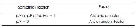
The ratio of the number of levels of a factor in an experiment to the potential number of levels in the population is called the sampling fraction for a factor. In terms of this sampling fraction, the definition of fixed and random factors may be summarized as mentioned in Table 1.
Table 1. Relationship Between Sampling Fraction and Fixed Random Factors
Cases in which the sampling fraction assumes a value between 0 and 1 do occur in practice. However, cases in which sampling fraction is either 1 or very close to 0 encountered more frequently. Main effects are defined in terms of parameters. Direct estimates of these parameters will be obtainable for corresponding statistic.
The main effect for the level is the difference between the mean of all potential observations on the dependent variable at the level and grand mean of all potential observations.
The interaction between different levels is a measure of the extent to which the criterion mean for treatment combination cannot be predicted from the sum of the corresponding main effects. From many points of views, the interaction is a measure of the non- additivity of the main effects. To some extent, the existence or nonexistence of interaction depends upon the scale of measurement. For example, the interaction may not be present in terms of a logarithmic scale of measurement, whereas in terms of some other scale of measurement an interaction may be present. If alternative choices are present, then that scales which leads to the simplest additive model will generally provide the most complete and adequate summary of the experimental data.
From literature survey, it is found that voltage, current, speed of arc travel and, Nozzle to Plate Distance, Gas Density (Manoj Singla, Dharminder Singh, & Dharmpal Deepak, 2010) are the parameters influencing the weld deposit area. So in the present work, these five variables are treated as treatment variables.
For conducting trial runs values or levels of these variables were chosen randomly from an infinite potential level i.e. the sampling fraction for these trials runs was equal to zero, however, has been obtained a rough range for these factors from the literature. With the help of these trial runs, effective representative's levels were developed for each factor (variables).
The numbers of levels for each factor included in the experiment are chosen as per the design. These numbers of levels were two for each so as per the definition it is a 2n (2*2*2*2) factorial experiment, where n is number of factors. If full factorial approach had been practiced, the number treatment combination would have been 32. But without affecting the accuracy of the model and the objective of the test, is carried out half factorial approach according to which, the number of treatment combinations becomes 2n-1(25-1= 24 = 16). The levels for each factor were the highest value and the lowest value of the factors inbetween and at which the outcome was acceptable. These values were outcomes of trial runs. Highest value has been represented by '+' and the lowest value has been represented by '-' as mentioned in Table 2. As per the design matrix, the final runs were conducted and the response i.e. the weld deposit area was measured and noted down against each combination.
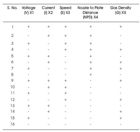
Table 2. Computations of Coefficients
Then the values of different coefficients were calculated as per the modeling. These values of coefficients represent the significance of corresponding factors (variable) on the response.
Higher the value of coefficients, higher the influence of the variable on response. Negative value of coefficients indicates the inverse relationship between variable and response. Computations of coefficients were done according to the model in Table 2.
Assuming the values of responses as y1, y2, y3, y4, … …. y16 against the treatment combinations 1, 2, 3, ……., 15, 16 respectively (as per the S. No. in the matrix design) Y as the optimized value of response (i.e. left hand side in the equation used for the showing the relation among the factors and the response).
Relation between main effects interactions effects and the response are shown in the following equation,
Y=b0 +b1 X1 +b2 X2 +b3 X3 +b4 X4 +b5 X5 +b12 (X1 X 2)+b13 (X1 X3 )+b14 (X1 X4)+b15 (X1 X5 )+b23(X2 X3 )+b24 (X2 X4 )+b25 (X2 X5 )+b34 (X3 X4 )+b35(X3 X5 )+b45 (X4 X5 )+b123 (X1 X2 X3 )+b124 (X1 X2 X4 )+b125 (X1 X2 X5 )+b134 (X1 X3 X 4)+b135 (X1 X2 X5 )+b145 (X1 X4 X5 )+b234 (X2 X3 X4 )+b235 (X2 X3 X5 )+ b245 (X2 X4 X5 )+b345 (X3 X4 X 5)
Here Y is the optimized weld deposit area, yi (i = 1 to 16) is the response of the ith treatment combination, b0 is the mean of all the responses, bj(j =1 to 5) is the coefficient of jth main factor (j= 1 for voltage, 2 for current, 3 for speed, 4 for NPD, 5 for gas density), and bjkl (j, k=1 to 4, l=0 to 5) is the coefficient for interaction factor.
Optimal values of treatment variables obtained by using the half factorial approach are presented in Table 3.
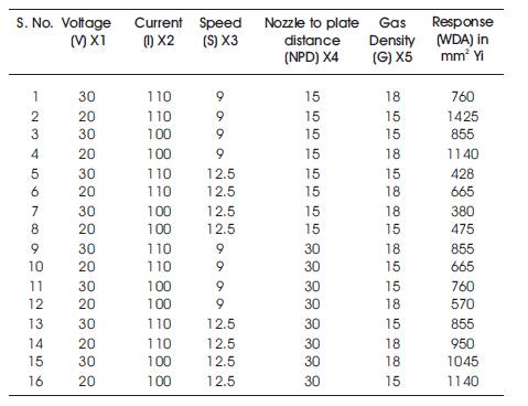
Table 3. Optimized Gas Metal Arc Welding Parameters
Now as per the equations mentioned earlier the values of different effects can be calculated as below:
b0 = 810.5, b1 = -68.25, b2 = 14.875, b3 = -68.25, b4 = 44.50, b5 = -14.875, b12 = 1.0750, b13 = 0.9875, b14 = 0.9875, b15 = 32.625, b23 = -32.625, b24 = -38.625, b25 = -3,b34 = 210.75, b35 = 32.625, b45= 14.875, b123 = - 32.625, b124 = 32.625, b125 = 68.25, b134 = -74.25, b135 = -14.875, b145 = 38.625, b234 = -38.625, b235 = 68.25, b245 = 74.25 ,b345 = -32.625
Now, the actual model can be represented as the following equation,
Y = 810.5+ (-68.25)X1 +(14.875)X2 +(-68.25) X3 + (44.5)X4 + ( -14.875)X5 + (- 32.625)(X1X2)+(3)(X1X3) + (92)( X1X4 ) + (32.625)(X1X5) + (32.625)(X2X3) + (-38.625) (X2X4 )+(-3)(X2 X5 )+(210.75)(X3 X4 )+(32.625)(X3 X5 )+ (14.88)(X4 X5 )(-32.625)(X1 X2 X3 )+(32.625)(X1 X2 X4 )+(68.25) (X1 X2 X5 )+(-74.25)(X1 X3 X4 )+(-14.875)(X1 X3 X5 )+(38.625) (X1 X4 X5 )+(-38.625)(X2 X3 X4 )+(68.25)(X2 X3 X5 )+(74.25) (X2 X4 X5 )+(-32.625)(X3 X4 X5 )
The graphical representation of the obtained relationship is shown in Figure 1.
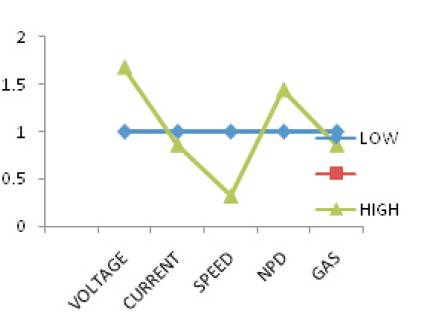
Figure 1. Graphical Representation
Graph in Figure 1 shows the weld deposition area is standardized with low level as the base and the variations thus coming are observed. So the graphical study thus indicates that voltage and speed varies directly with the weld deposit area, and current and NPD and gas density varies inversely.
Here, as per the graph, there is an overall variation of about 60% in direct relation with voltage and 68% inverse relation with speed and exists an overall 15% inverse variation with respect to current and 44% variation with NPD and negotiable inverse relationship with gas density. Therefore, it is clear that, it is highly preferable to operate welding at lower levels of voltage and speed and current and NPD at higher levels.
So thereby to compensate all the kind of ills occurring during the welding process, it is necessary to make the adjustments of these all variables with the low level value reference i.e., the voltage value is directly proportional to weld deposit area which states that the base low level increasing can give better possible weld depositions.
The mixed coefficient of variables gives a common interaction coefficient which in turn becomes a relative variable coefficients. And they are inter related on one another interactions.
The strength of the weldment largely depends on the weld bead area. Here the authors are aiming at increasing the weld bead area by carefully setting the best optimal parameters. Hence, clearly the strength of the weldment is increased.
Material used: Ferron 6013
Composition: Carbon 0.1%, Manganese 0.6%, Silicon 0.3%, Sulphur 0.03%, Phosphorus 0.03%.
The following are the best possible strength values of the products manufactured at the industry.
Ultimate tensile stress: 550 N/mm2
Yield strength: 440 N/mm2
Now these are the values that have been obtained by optimal parameters in this study:
Ultimate tensile stress: 527 N/mm2
Yield strength: 418 N/mm2
If the same analysis is carried out by setting some random values of the parameters, the results obtained are as follows:
Ultimate tensile stress: 463 N/mm2
Yield strength: 393 N/mm2
Clearly by comparing the above results, it is evident that the study carried out by setting the optimal parameters has successfully yielded good properties of the weldment. As a result of this, the aim of the analysis has been successfully achieved.
In the present work the various factors which influence the weld deposit area are identified and their quantitative influence on the same was investigated. Results indicate that process variables are influencing the weld bead area to a significant extent. Among the variables taken into consideration Welding current was found to be most influencing variable influencing the weld deposit area. Weldments made by taking into account inputs like constant heat input, electrode negative polarity (DCEN), electrode with small diameter, long electrode extension, low voltage and low welding speed are producing a large weld bead area. It is also observed, that two level fractional half area fractional designs is found to be very efficient tool for quantifying the main and interaction effects of variables on weld bead area.