(1)
A numerical technique for solving time and robust time-optimal control problems has been presented. The method relies on the special feature that the optimal control structure contains as many free parameters as there are interior or boundary conditions. Two Boundary Value Problems (BVPs) are formulated for the state variables and co-states independently, thus, reducing the dimension of the original problem into half. Then, a numerical algorithm is developed, that is based on the shooting method, to solve the resulting BVPs. The computed optimal solution is verified by comparing the control input resulting from the first BVP with the switching function obtained by solving the second BVP. Next, the numerical technique is modified to solve robust time-optimal control problems. The capability of the proposed method is demonstrated through numerical examples, whose output optimal solution is shown to be identical to those presented in the literature. These examples include linear as well as non-linear systems. Finally, the numerical technique is utilized to design a time-optimal control for a rest-to-rest maneuver of flexible structure while eliminating the residual vibrations at the end of the maneuver.
In recent years, there has been a considerable interest in modeling and control of flexible structures. This is due to the use of lightweight materials for the purpose of speed and fuel efficiency. Furthermore, many applications, such as robotic manipulators, disk drive heads and pointing systems in space are required to maneuver as quickly as possible without significant structural vibrations during and/or after a maneuver.
The time-optimal control for general maneuvers and general flexible structures has posed a challenging problem and is still an open area for research. In particular, the time-optimal control for rest-to-rest slewing maneuvers of flexible structures has been an active area of research, and only limited solutions have been reported in the literature. Solution to the time-optimal control problem of a general flexible system is faced with two main obstacles. First, the number of control switching times is an unknown priori and must be guessed. Second, as the number of modes included in the model is increased, the computer time required by these numerical techniques becomes prohibitive.
In the recent literature, many researchers [1-7] have developed computational techniques that deal with solving time-optimal control of flexible structures. In all of these works, the exact time-optimal control input, which is of the bang-bang type, is calculated based on transforming the time-optimal control problem into parameter optimization.
The paper presents a numerical technique to solve a general time-optimal control problem. The basic idea of the approach is to transform the necessary conditions of optimality into two boundary value problems (BVPs), which involve the states and co-states separately. Consequently, a large saving in computer time is gained with the proposed approach. The method depends on the special feature that the optimal control structure contains as many free parameters as there are interior or boundary conditions for the state variables [8].
At first, the paper introduces the numerical technique by applying it to a benchmark problem. Then, the numerical technique is modified with the purpose of computing a robust time-optimal control input. This is followed by, applying the method to a non-linear system, proving the method to be applicable to linear as well as nonlinear systems. The design of a time-optimal control input for a flexible structure with one rigid body mode and ten flexible modes has been presented in the next section. This is followed by some concluding remarks.
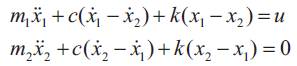
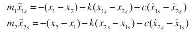
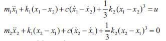
To introduce the proposed control design technique, the control of a two-mass-spring-damper system has been considered as shown in Figure1, which has one flexible mode and one rigid body mode. The equations of motion are
where x1 and x2 represent the displacement of the first and second masses respectively. Transfering this system from the initial conditions,

to the final conditions,

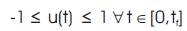
and subject to the control magnitude constraints,
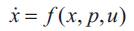
in minimum time. This system can be written compactly in state space form as,
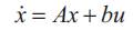
where x = [ x1 x2 x3 =dx1 /dt x4 =dx2 /dt]T is the state vector, and
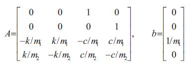
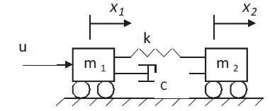
Figure1. Mass-spring-damper system
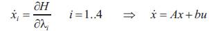
The necessary conditions of optimality can be derived by defining, first, the Hamiltonian H as,

where λi=1..4 are the co-states (Lagrange multipliers).
The necessary conditions of optimality require the following equations to be satisfied.
1. The state equations,
2. The co-state equations,
3. The boundary conditions, Equations 2.
4. The transversality condition for the free end time tf yields
5. The time-optimal control u(t) minimizing the Hamiltonian H is,
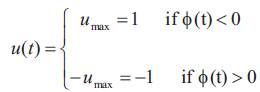
where φ(t) = ∂H/∂u = λ3(t) is the switching function for the control input u(t). It can be shown that the system in Equation 4 is normal [9], [10], a property that eliminates the existence of singular intervals and forces the necessary conditions to also be sufficient. Therefore, the control is of the bang-bang type, as given by Equation 10, which can be parameterized by its switch times. Many researchers [1-5] have noted that the time-optimal bang-bang solution for a spring-mass-damper dynamical system with n degrees of freedom and with the type of maneuver described by Equation 2 (i.e., a rest-to-rest maneuver) has, in most cases, 2n -1 switches. Consequently, for two degrees of freedom system, the above necessary conditions of optimality can be put into a BVP with the twelve variables, x1, x2 , x3, x4, λ1, λ2, λ3, λ4, ts1, ts2, ts3 and tf as the unknowns with twelve boundary and interior conditions, eight boundary conditions in Equation 2, three switching conditions, λ3(t) = 0 at t = ts1, ts2 and ts3 , and the transversality condition, Equation 9, applied at either t = 0 or t = tf . Many researchers have developed numerical techniques to solve the above BVP.
Lastman [11] and Li [12]have used the shooting method to arrive at the time-optimal solution. Other researchers [1-6]have transformed the time-optimal control problem into constrained parameter optimization problem. The basic idea for this transformation is to assume a number for the control switch times, integrate the system equations, Equation 7, and imposing the boundary conditions, Equation 2. The resulting nonlinear equations, which are functions of the control switch and final times, are used as constraints in the parameter optimization problem. Therefore, the resulting constrained parameter optimization problem, for the system in Equation 7, is to determine the four parameters, ts1 , ts2 , ts3 and tf , that minimize the maneuver time tf , and subject to the four nonlinear equations resulting from applying the control structure, shown in Figure 2, to the system in Equation 7. Since the formulation of the parameter optimization problem does not depend on the necessary conditions of optimality, the resulting solution needs to be verified for optimality. This is accomplished by checking if the resulting solution satisfies the necessary conditions of optimality. Ben Asher [2] has proposed a numerical technique to verify the optimality of a solution resulting from a parameter optimization problem.
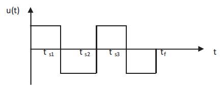
Figure 2. Time-optimal control structure
The numerical technique introduced in this paper is to formulate a BVP involving only the state variables by using the fact that optimal control problem contains as many free parameters as there are interior or boundary conditions. A second BVP which involves only the co-states is also formulated and solved to verify the optimality of the state space solution, resulting from solving the first BVP. Consequently, the numerical complexity of the original time-optimal control problem is reduced considerably with this approach. A numerical algorithm is outlined to solve both BVPs by using the shooting method.
The formulation of the BVP depends, first, on knowledge of the optimal control structure. For the above example, if the control structure, shown in Figure 2, is believed to be time optimal then, the resulting BVP has the eight variables, x1 , x2 , x3 , x4 , ts1 , ts2 , ts3 and tf . The boundary conditions necessary to solve this BVP are the eight boundary conditions stated in Equation 2. The second BVP contains the four variables,λ1,λ2,λ3 and λ4 as unknowns with the three interior conditions, λ3(t) = 0 at t = ts1 , ts2 and ts3 , and one boundary condition, which is the transversality condition applied at either t = 0 or t = tf .
In this paper, a simple numerical technique is proposed to solve the BVP formulated. The method is based on the simple shooting method, and is applicable to any general BVP. The numerical procedure is illustrated in the following steps:
Step 1: Assume starting values for the unknowns. In our example, these are the control switch and final times, ts1, ts2 , ts3, and tf .
Step 2: Integrate the state equations, Equation 7, from t = 0 to t = tf , using the initial conditions in Equation 2a, the control structure shown in Figure 2 and the assumed values for the control switch and final times.
Step 3: Form the vector of errors,
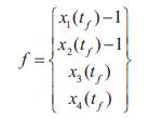
It is obvious, that when all the components of the vector f become equal to zeros, then all the boundary conditions are satisfied and we hope that we arrive at the optimal solution.
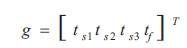
Step 4: Calculate the Jacobian matrix,
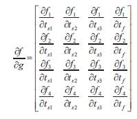
where fi and gi=1...4, are the i-th component of the vectors f and g. The vector g is defined by,
The above Jacobian matrix can be calculated either analytically or numerically using, for example, finite difference. Analytical derivatives can be calculated by integrating, symbolically, the state equations, Equation 7, using the control structure, shown in Figure 2, Then differentiate the resulting equations with respect to the control switch and final times.
Step 5: Perform the computation,
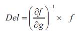
where Del is a 4 X 1 vector representing the step direction with which the control switch and final times should change in order for the components of the vector f to reach zero.
Step 6: Update the unknown variables using the equations,
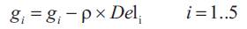
Where (.) is the i-th component of (.), and ρ is a constant representing the step size. As a general guide, the value of the constant ρ should be between zero and one to avoid divergence.
Step 7: Repeat Steps (1) - (6) until,
Norm (f) ≤ tolerance
where norm refers to the Euclidean norm of the vector f, and tolerance is a specified small number affecting the accuracy of the resulting solution.
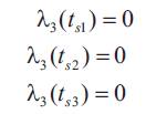
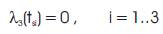
Once the optimal solution for the state variables and the control switch times are calculated, the corresponding time-optimal solution for the co-states is computed. A BVP involving the co-states can be formulated with the help of the necessary conditions of optimality. It involves solving for the four unknowns λ1(0),λ2(0),λ3(0) and λ4(0) given the three interior conditions,
and the transversality condition , Equation 9, applied at the final time tf ,
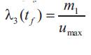
where umax is the maximum value for the control input, taken here to be one.
The same numerical procedure outlined above can be used to solve for the co-states by replacing the vectors g and f with the corresponding vectors of unknowns and errors, respectively.
For m1= m2= k = 1, and c = 0, the above numerical algorithm is programmed in Matlab, where the derivatives in Equation 12 is calculated using the finite difference equations,
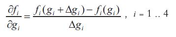
The resulting time-optimal control switch times, in seconds, are presented in Table 1.
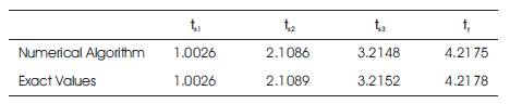
Table1. Computed and exact control switch times
The corresponding numerical values for the parameters used and the number of iterations with which the algorithm is able to reach the time-optimal solution are shown in Table 2.
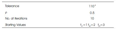
Table 2. Parameter values used in the algorithm and number of iterations
Table 1 shows that the resulting time-optimal control profile is identical to those listed in the literature. The numerical simulation for the states, and control input u(t) and switching function λ3(t) are shown in Figures 3 and 4 respectively.
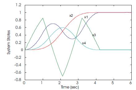
Figure 3. Response of a spring-mass-damper to a time-optimal control input
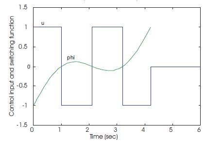
Figure 4. Control input u(t) and switching function = λ3(t)
It is well known [13] that, the resulting time-optimal solution calculated, is very sensitive to plant modeling uncertainty. The resulting time-optimal control, from the preceding example, is applied to the system of Equation 7. While changing the value of the stiffness from k = 1 to k = 1.1, 1.2 and 1.3, then the resulting system trajectories is shown in Figure 5, where it is seen that small changes in the value of k (10%~30%) resulted in a large increase in the vibrational amplitude of the flexible mode. Therefore, there is a need to design a robust time-optimal control input that reduces the sensitivity of the optimal solution for modeling errors. In particular, we would like to minimize the sensitivity of the final states of a dynamic system, to errors in the estimated parameters of the system. Following [13], we consider a general system represented by the state equation,
where x is the state vector of the system, p is a parameter vector and u is the control input. To determine the sensitivity of the final states of the system to a change in the parameter vector ρ, we could use the finite difference approximation for the derivatives as,
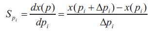
where the subscript i denotes the ithparameter of interest. Evaluating Spi at the final time provides us with an estimate of the sensitivity of the final states to a change in the parameter pi. Alternatively, and more accurately, the state I sensitivities could also be evaluated by the direct differentiation of the state equation as,
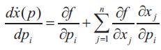
Integrating Equation 17 along with Equation 18 leads to the sensitivity of the states to the parameter pi .
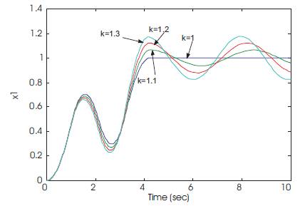
Figure 5. Response to time-optimal control
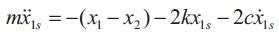
Now, let us consider designing a robust time-optimal control input for the system in Equation 1. Applying Equation 19 to the system defined by Equation 7 for the sensitivities of x1 and x2 to the parameter k leads to,
where x1s=∂x1/∂k and x2s=∂x2/∂k are the sensitivities of x1 and x2 to a change in the parameter k. From Equation 20, for m1 = m2 = m , then
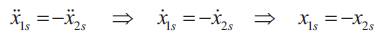
and, therefore, one of the sensitivities can be eliminated to give
Then, the augmented state equations are the system equations, Equation 7, and the state space form of Equation 22. The augmented boundary conditions are the original boundary conditions, Equation 2, and,

It is clear that the boundary conditions in Equation 23 force the sensitivities of the state’s x1 and x2 at the final time to zero. Now the objective is to design a control input u(t) that minimizes the final time tf , subject to the state equations, Equation 1 and 22, the control constraints, Equation 3, and the boundary conditions, Equation 2 and 23. Since we have added the robustness constraint, represented by Equation 22, in the formulation of the BVP, then the number control switches must be increased to match the number of constraint equations. In [1] and [3], it has been shown that adding the robustness constraint, Equation 22, increases the number of time-optimal control switches by two.
Therefore, the resulting BVP has the twelve variables, x1 , x2 , x3 , x4 , x1s , dx1s /dt, ts1 , ts2 , ts3 , ts4 , ts5, and tf , with twelve boundary conditions, eight boundary conditions, Equation 2 and the four boundary conditions, Equation 23. It is noted that the number of control switch times has increased by two [1],[3], emphasizing the fact that the number of variables should match the number of boundary and interior conditions.
The numerical algorithm is applied to solve for the robust time-optimal control problem, with the same parameter values used in the preceding example, m1 =m2 =k=1 and c=0. The resulting control switch times, in seconds, are presented in Table 3. In addition, the numerical simulation for the displacement x1 is shown in Figure 6. It can be seen that the application of the robust time-optimal control to a system with error in the stiffness value has reduced the residual vibration significantly.
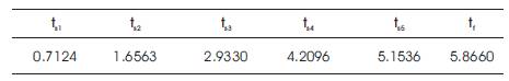
Table 3. Robust time-optimal control switches times
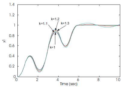
Figure 6. Response to robust time-optimal control
This section demonstrates the capability of the proposed numerical algorithm to solve for the time-optimal control of nonlinear systems. Again, consider the two-mass-spring damper system, with nonlinear spring element representing hard spring characteristics [13]. The equations of motion are,
For a rest-to-rest maneuver, we assume the same boundary conditions as those given by Equation 2.
It is desired to perform a minimum time maneuver for the system of Equation 24, subject to the control constraints, Equation 3, and satisfying the boundary conditions, Equation 2. The necessary conditions of optimality can be derived easily as follows.
Assuming the number of time-optimal control switches to be three, the resulting BVP has the eight variables, x1 , x2 , x3 , x4 , ts1 , ts2 , ts3 , and tf along with the eight boundary conditions, Equation 2. Similarly, the BVP for the co-states contains the four variables, λ1,λ2,λ3,λ4 along with the three switching conditions,
And the transversality condition applied at the final time

It is noted that the costate equations can be derived easily using Equation 8.
The numerical algorithm is applied to this example, with k1 =k2 =m1 =m2 =1 and c=0, to calculate the time-optimal control input. The system response to the time-optimal control input is shown in Figure 7, whereas, the control input and switching function λ3(t) are shown in Figure 8. Similarly, it is straight forward to calculate the robust time-optimal control input with respect to changes in either k1 or k2 using similar procedure as for the linear example treated earlier.
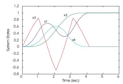
Figure 7. Nonlinear system response to time-optimal control
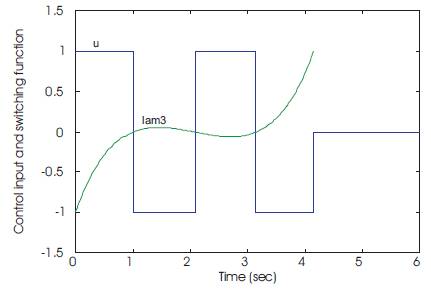
Figure 8. Time-optimal control for nonlinear system
As an example to illustrate the numerical procedure and show its effectiveness, we consider the time-optimal single axis maneuver problem for a system consisting of a rigid hub with two uniform elastic appendages attached to it. A single actuator that exerts an external torque on the rigid hub controls the motion of the system. It is desired to rotate the flexible system by 90 degrees as quickly as possible while suppressing the vibration at the end of the maneuver to achieve good pointing accuracy.
For comparison purposes, we use the same material and maneuver specifications that are used in [4], and are shown in Table 4.
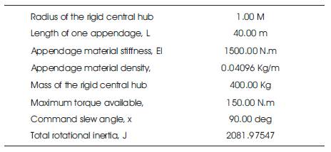
Table 4. System dimensions, appendage material, and maneuver specifications
The Euler-Bernouli beam assumption is made to obtain the equations of motion for the system. It is assumed further that the beam is inextensible, in the sense that the stretch of the neutral axis is negligible, and no structural damping is present. The assumed mode method based on modal expansion is applied to the two flexible appendages, where the rigid body mode and the first 10 vibrational modes are retained in the evaluation model. The normalized mode shapes for a fixed-free cantilever beam are used as the assumed mode shapes. The discretized equations of motion, in matrix form, are,
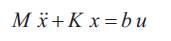
where x, and b are 11 x 1 vectors and M and K are 11 x 11 matrices. Using the matrix of eigenvectors, normalized with respect to the mass matrix, the system in Equation 27 is transformed to,
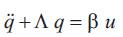
using the transformation,

where Λ is an 11x11 diagonal matrix with the diagonals being ωi2 , i = 0 .. 10, and φ is 11X11 matrix of eigen vectors. Table 5 shows the natural frequencies ωi and the modal participation vector components βi(β=φTb).
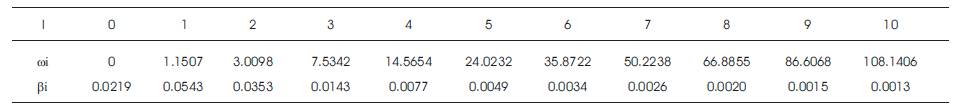
Table 5. Modal Quantities
Using the numerical technique we first design a time optimal control input for the rigid body mode. Then the number of modes in the time-optimal control calculations is increased until the flexible system is rotated with the smallest error while minimizing the structural vibrations at the end of the maneuver. The time-optimal control switches and final times for the rigid body mode, rigid body mode and one flexible mode, and rigid body mode and two flexible modes are presented in Table 6. The rigid hub attitude response for the three time-optimal control inputs, designated by u1,u2 and u3, are shown in Figure 9. As seen from the figure, the control input designed for the rigid body mode and two flexible modes is able to perform the maneuver in minimum time, while eliminating the residual energy at the end of the maneuver.
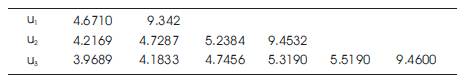
Table 6. Time-optimal control switch and final times
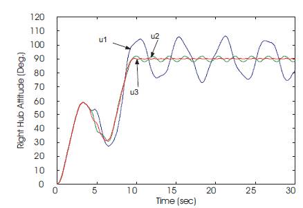
Figure 9. Rigid hub attitude
This paper outlined a new numerical algorithm to calculate both time- and robust time-optimal control problems for linear as well as nonlinear systems. The algorithm relies on formulating and solving a BVP, derived from the necessary conditions of optimality that contains the state variables and co-states, separately, resulting in smaller dimensional problem. A numerical procedure is outlined to solve, based on the shooting method, the resulting BVP. The algorithm is first tested by solving a benchmark problem (mass-spring-damper system) and the resulting time- and robust time-optimal control is shown to be identical to that presented in the literature. Then, the numerical technique is used to solve the time-optimal control design for a nonlinear system. Finally, the algorithm is utilized to design a minimum time control input for a flexible structure without causing any residual vibrations at the end of the maneuver.