Demand forecasting is an important aspect of business operation. Also proper demand forecasting allows for more efficient and responsive business planning. There are two general approaches to forecast: qualitative and quantitative. Qualitative methods consist mainly of subjective inputs, which often defy numerical description. Quantitative methods either involves the extension of historical data or the development of associative models that attempt to utilize causal (explanatory) variable to make a forecast. Quantitative method is a time-ordered sequence of observation taken at regular intervals over a period of time (e.g. hourly, daily, weekly, monthly, quarterly, annually). The data may be measurements of demand, earnings, profits, shipments, accidents, output, precipitation, productivity and consumer price index. Forecasting technique based on time series data are made on the assumption that future values of the series can be estimated from past values.

Qualitative techniques permit inclusion of soft information (e.g., human factors, personal opinions, hunches) for the forecasting process. These factors are often omitted or downplayed when quantitative techniques are used because they are difficult or impossible to quantify. Quantitative techniques mainly consists of analyzing objective or hard data.

Exponential smoothing is one the time series technique which is widely used for forecasting. Exponential smoothing is a sophisticated weighted averaging method that is still relatively easy to use and understand. Each new forecast is based on the previous forecast plus a percentage of the difference between that forecast and the actual value of the series at that point.

In a literature survey, Sahu and Kumar, (2013) introduced the demand fluctuation of dairy products and the forecasting practices that have been used by Raipur Dugdh Sangh (Devbhog Dairy Iindustry) in Chhattisgarh. They used various types of forecasting methods like single Moving Average Method (SMA), Double Moving Average Method (DMA), Single Exponential Method (SEM), Double Exponential Method (DEM), Semi Average Method (SAM) and Naive Method. Based on the accuracy, Single Exponential Smoothing (SES) method with α=0.3 produces the most accurate forecasting.

Cacatto et al., (2012) included the forecasting practices that have been used by food industries in Brazil and detected how these companies have been using this forecasting methods, and what are the main factors that influence their choice. The data was analyzed by multivariate statistics techniques using SPSS software. The result shows that the companies do not use sophisticated forecasting methods; but use the historical analysis models. The factors that influence the selection of these models are, type of product, time spent during forecasting, and the main drawback is the availability of the appropriate software.

Lim and Nayar, (2012) analysed of the predictions for solar irradiance and load demand using two different Single Exponential Smoothing forecasting approaches. Both the approaches perform prediction based on hourly basis. The first approach uses the current day’s data while the other uses the previous day’s data. Comparison between the two approaches are carried out, and the forecasting result shows that the Single Exponential Smoothing forecast models utilizing the previous day’s data has achieved higher accuracy than that of the previous hour data.

Paul, et.al., (2011) addresses the selection of optimal value of exponential smoothing constant to minimize the Mean Square Error (MSE) and Mean Absolute Deviation (MAD). Trial and error methods is used to determine the optimal value of exponential smoothing constant.

Ravinder, et.al., (2013) examined the impact of initial forecasts on smoothing constants with the idea of optimizing these initial forecast along with the smoothing constants. They make recommendations on the use of Solver method in context with the teaching of forecasting and suggested there is a better method than Solver to identify the appropriate smoothing constants.

Hyndman (2002) provided a new approach for automatic forecasting, based on an extended range of exponential smoothing methods.

Corberan-Vallet et al. (2011) presented the Bayesian analysis of a general multivariate exponential smoothing model that allows to forecast time series jointly, subject to correlated random disturbances.

While Taylor, et.al.,(2003) investigated on a new damped multiplicative trend approach. An empirical study on using the monthly time series from the M3-Competition, gave encouraging results for the new approach at a range of forecast horizons, when compared to the established exponential smoothing methods.

Strasheim, (1992) stated that the exponential smoothing method is a technique that uses weighted moving average of past data as the basis for a forecast. This method keeps a running average of demand and adjusts it for each period in proportion to the difference between the latest actual demand figure and the latest value of the average. The equation for the simple exponential smoothing method is,

F_t+1 = α Y_t + (1-α) F_t-1

where:

F_t+1 - new smoothing value or the forecast value for the next period.

α - Smoothing constant (0 < α <1)

Y_t - new observation or actual value of the series in period t

F_t - old smoothed value or forecast for period t

Mean Square Error

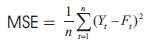
Chary, (2009) and Panneerselvam, (2009) stated that the Mean Square Error (MSE) is the squares of the deviations of the forecast demands from the actual demand values. This method of measuring errors that penalizes large errors more than small errors is sometimes required.

The equation is given as,

 

where:

Y_t - the actual value in time period t

F_t - the forecast value in time period t

n - the number of periods

A common method for measuring overall forecast error is Mean Absolute Deviation (MAD) method. Ryu and Sanchez, (2003) and Chopra and Meindi, (2010) noted that this value is computed by dividing the sum of the absolute values of the individual forecast error by the sample size (the number of forecast periods). The equation is,

 

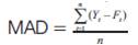
where:

Y_t - actual value in time period t

F_t - forecast value in time period t

n - number of periods

The data for this study were collected and recorded on weekly basis. The data contains sales of product (paneer) from October 2011 to October 2012. All the data was saved in an Excel spreadsheet.

The method is described by considering a problem. A company's historical sales data are given for some previous periods. Actual values of sales are given in Table 1.

For different values of exponential smoothing constant, MSE and MAD are calculated. Mean square error for different values of exponential smoothing constant are determined using the equation. Table 2 shows the MSE values for different α.

Mean absolute deviation for different values of exponential smoothing constant are determined using equation. Table 3 presents the MAD values for different α.

Values of MSE and MAD are differed with the values of α. MSE is decreased with increasing α value upto 0.52 and after which MSE increases. Variation of MSE with a is shown in Figure 1. MAD is decreased with increasing a value upto 0.60 and later MAD is increased. Variation of MAD with α is shown in Figure 2. The value of exponential smoothing constant is 0.52 and 0.60 for minimum MSE and MAD respectively.

To find the optimal value of exponential smoothing constant, minimum values of MSE and MAD are selected and this corresponding value of exponential smoothing constant is the optimal value for this problem.

Minimum values of MSE and MAD and the corresponding value of exponential smoothing constant is given in Table 4.

From the optimal value of α, forecast values for different period are determined and it is shown is Table 5. From the fifty six period actual values, a sale at fifty seven period is also forecasted. Forecasts at fifty six periods are 12.455 thousand and 12.068 thousands for minimum MSE and MAD respectively.

Figure 3 represents the actual demand, compared to the corresponding forecast values of mean square error and mean absolute deviation.

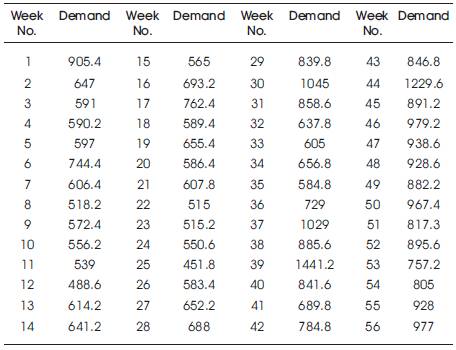
Table 1. Demand of product (paneer) (in kg)

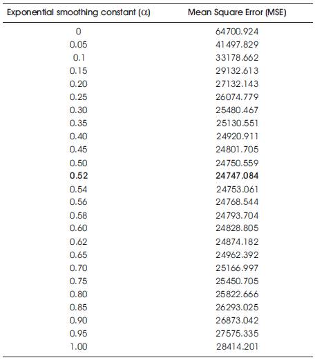
Table 2. MSE for different values of α

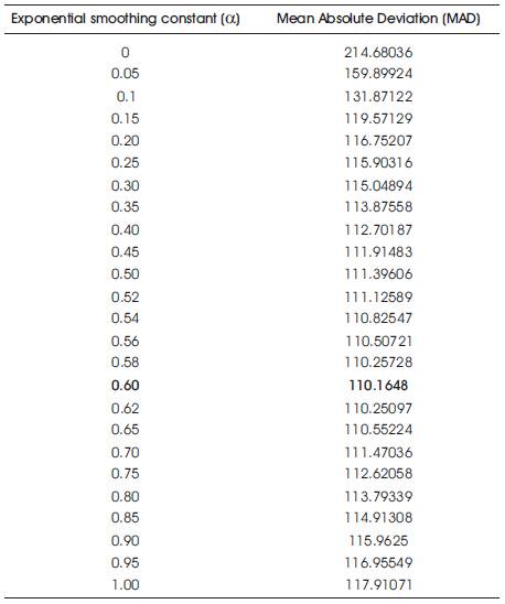
Table 3. MAD for different values of α

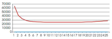
Figure 1. Variation of MSE for different values of α

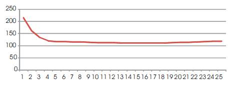
Figure 2. Variation of MAD for different values of α

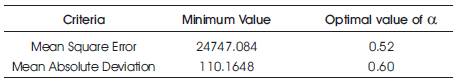
Table 4. Optimal Values of a for minimum MSE and MAD

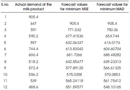
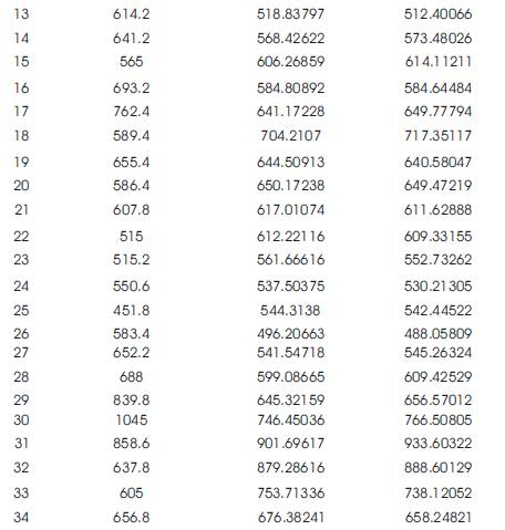
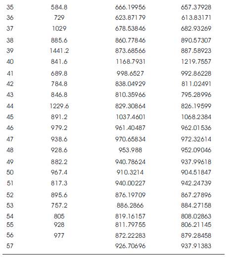
Table 5. Forecast values for minimum MSE and MAD

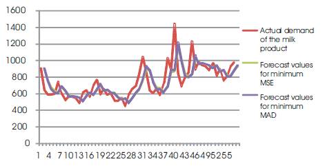
Figure 3. Comparison of Actual Demand & Forecast Demand

For checking the validation of single exponential forecasting method, apply single exponential forecasting method with α=0.52, 0.60 for the weekly data from 1 November 2012 to 15th May 2013.

Figure 4 shows the graph between the actual demand of milk product, Forecast value for minimum MSE (α=0.52) and Forecast value for minimum MAD (α=0.60). The difference between the actual demand of milk product and forecast demand with smoothing constant value 0.52, 0.60 are small.

Table 6 showed that Single Exponential Method with α=0.52 obtained the error 3.34% and Single Exponential Method with α=0.60 obtained the error 2.76% ; however, both the values of a provides minimum error and this method is selected as the most appropriate forecasting method for sales forecasting of milk product (Paneer) in Chhattisgarh, India.

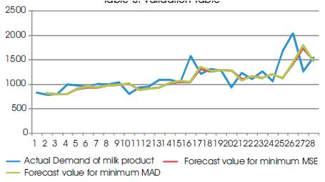
Figure 4. Validation Graph

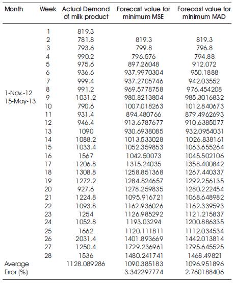
Table 6. Validation Table

Exponential smoothing technique is one of the most important quantitative techniques used in forecasting. The accuracy of this forecasting technique depends on exponential smoothing constant. Choosing an appropriate value of exponential smoothing constant is very crucial for minimizing the error in forecasting. In this paper, future demand of the milk product (Paneer) is estimated by determining the optimal value of exponential smoothing constant. Mean Square Error and Mean Absolute Deviation are minimized to get the optimal value of the constant and optimal values 0.52 and 0.60 for Minimum Mean Square error and Mean Absolute Deviation respectively. In this method, Raipur Dugdh Sangh (Devbhog) can compute the optimal value of α=0.52, 0.60 for exponential smoothing constant to enhance the accuracy of demand forecasting of milk product (Paneer). This work can be extended for minimizing forecast errors such as Mean Absolute Percent Error (MAPE), Cumulative Forecast Error (CFE) etc.