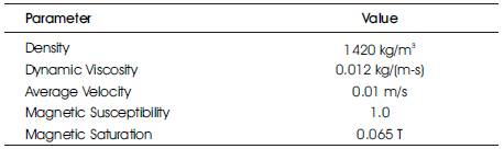
Table 1. Physical Properties
Numerical simulations of ferrofluids are carried out in two-dimensional and three-dimensional space in order to analyze the magnetic effects on flow behavior for magnetic drug targeting (MDT) applications. MDT is a novel technique that allows the concentration of drugs to be guided to a defined target region (TR) with the help of a magnetic field, made possible by the magnetic property of the fluid itself. Ferrofluids are two-phase solutions composed of magnetic nanoparticles suspended in a carrier fluid. Ferrofluids are modeled in a pipe geometry with a sphere-shaped target site and magnetic effects are modeled as fields resulting from current carrying wires. Parameters that are studied include different strengths and locations of magnetic field. Pressure distributions and velocity contours particularly in the TR show the added flow recirculation and increase in the fluid's retention time at the TR, due to the magnetic field. Furthermore, the studies presented here provide a fundamental understanding of the behavior of a magnetic fluid, modeled here as a single-phase fluid thereby affirming the feasibility of such fluids in MDT applications with regard to enhanced drug transfer.
There have been numerous advancements in developing a suitable methodology of administering drug molecules to a localized area of concern within the body, without negatively impacting healthy surrounding tissues, especially in the medical treatment of various diseases such as cancer, thrombosis, aneurysms, and atherosclerosis. Magnetic Drug Targeting (MDT) is one such technique. MDT allows the concentration of drugs to be guided to a defined target site with the help of a magnetic field. Typically the drug compound is bound with magnetic nanoparticles and is injected through the blood vessels thus supplying the target tissue with the necessary medicine, all in the presence of an external magnetic field. It is believed that the increased interaction of the drug molecules with the desired site is the underlying reason why MDT delivery techniques are advantageous over conventional techniques [1]. Typically, this is achieved once the ferrofluid and drug mixture are injected into the body, and the magnetic field strength and gradient are strong enough to maintain the drug molecules in the location of the desired region long enough to produce the desired results.
Ferrofluids, which are a two-phase solution composed of magnetic nanoparticles suspended in a carrier fluid, are of specific interest due to their high magnetic moment and biocompatibility [2]. Ferrofluids have particles on the nano-scale and their Brownian motion keeps the particles from settling or clumping together. When introduced to a magnetic field, the fluid becomes magnetized and a magnetic moment is generated [3]. The first reported case of MDT delivery in humans was by Lubbe, et al, in 1996 [4]. Many aspects of MDT with ferrofluids are attractive, including the non-invasive nature of the procedure, the increased delivery of medicine to the target site, the decreased risk of potentially dangerous side effects due to the large amount of required drugs and the increased cost effectiveness of minimizing the amount of necessary drugs. Over the past 15 years MDT with ferrofluids has become increasingly promising with increased laboratory testing and simulation techniques. Due to the vast number of potential benefits, MDT delivery techniques continue to be an expanding, exciting area of research in universities and hospitals around the world.
An excellent review of the use of magnetic nanoparticles for drug delivery was provided in [1]. In the study of Jain et al.[5] a dynamic model of ferrofluids as drug carriers flowing in a blood vessel was formulated for magnetic drug delivery. Another clinical study [6] used iron oxide nanoparticles covered by starch derivatives with phosphate groups, and showed that a strong magnetic field gradient at the tumour location accumulates the nanoparticles. The objective of this research was to establish a fundamental understanding of the physics and the parameters involved in the design of a magnetic drug targeting system.
The physical problem considered in this study involves the flow of a ferrofluid in a pipe that has a circular depression for the drug-targeted region. The physical parameters that are considered in this study include the density and dynamic viscosity of both blood and the ferrofluid to be modeled, the magnetic susceptibility of the ferrofluid, the magnetic saturation of the ferrofluid, the typical diameter of an artery in the area of interest, the geometric characteristics of the Targeted Region (TR), e.g. an aneurysm, the average and maximum speed of blood flow both within an artery and within the TR. Ferrofluid properties for the fluid, Ferrotec EFH3, were used, and were obtained from Ferrotec, Inc. The EFH3 fluid was selected for its high magnetic saturation.
Table 1 shows the assumed physical parameters for the model.
The three dominant aspects that were adjusted to maximize retention of medicine molecules in the infected area were (i) the overall strength and orientation of the magnetic field, (ii) the selection and modeling of a ferrofluid to maximize response, (iii) and the selection of workable body regions, such as considering characteristics of blood velocity and vessel diameter.
Table 1. Physical Properties
The selected geometry is an idealization of anTRon the edge of a blood vessel. A similar geometry was used in the CFD simulations presented in [7]. In this study, the fluid has been modeled as a single-phase fluid with the magnetic effects being manifested entirely in terms of the Kelvin body force term given by
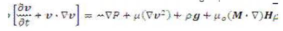
This body force is a source term in the momentum equation as follows:

The Kelvin body force term is basically a term that summarizes the projection of fluid magnetization onto magnetizing field [4]. In order to manipulate the controllable nature of the ferrofluid, the strength of the magnetization and the gradient of the magnetizing field can be adjusted. Physical constraints on the magnetization are limited by the fluid's magnetization saturation limit. Since the body force is proportional to the gradient of the magnetizing field a uniform field would induce no additional force on the fluid domain. The analytical theory related to the formulation of the equations, specifically with regard to the magnetic source terms is presented in Appendix 1.
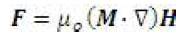
The commercial software ANSYS 12.1 along with FLUENT for fluid flow solutions, were chosen as the computational engine in this study. The physical problem consists of the flow of a ferrofluid as a single-phase fluid entering the inlet on the left and exiting the outlet on the right. The velocity inlet conditions for the computation are presented in Appendix 2. The pressure-based solver in ANSYS was employed to solve the steady-state Navier-Stokes equations, where a second-order upwind scheme was used to discretize the inertia terms. The grid resolution employed for the computational domain consists of 25,400 points. Tables 2 & 3 in Appendices 3 and 4 show the grid resolutions for the 2D and 3D computations, respectively. These appendices also show the analytical functions for the magnetic dipole. The Kelvin body force as an additional source term in the momentum equations is implemented into the code using the User Defined Function (UDF) feature of ANSYS FLUENT. All calculations were run on up to 4 processors on a AMD Opteron quad core architecture and typical CPU times were 2 - 4 hours per calculation. Figure 1 shows the schematic of the computational domain and Figure 2 shows the grid configuration.
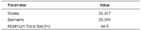
Table 2. 2D Mesh Parameter Values
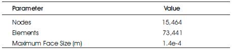
Table 3. 3D Mesh Parameter Values
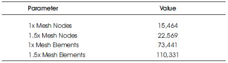
Table 4. 3D Mesh Parameter Values for Grid-Dependent Studies
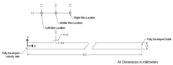
Figure 1. Schematic of the Geometry
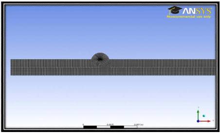
Figure 2. 2D Computational Mesh
The geometry inlet has been setup as a velocity inlet with a parabolic profile; justification for this parabolic profile is well documented as the laminar nature of blood flow in small diameter vessels. The geometry outlet condition is a fully developed surface, justification for which has been taken care of with a long uniform developing region greater than 30 diameters in length between the TR and the outlet. All walls of the model have been setup as rigid walls with a “no slip” condition. This simplification may be an unrealistic model of biomedical simulation but is a necessary assumption since the focus of this paper is on the effect of various magnetic fields on the flow of ferrofluids for such medical applications.
In an attempt to develop a versatile code the magnetizing field has been assumed to be of the form as follows.
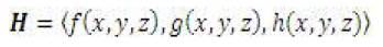
The code developed reads an input text file which holds the coefficients for the above field to generate any field, which is sufficient to model uniform gradient fields and current carrying wire fields.
This section presents the results of the 2D and 3D simulations conducted as part of the effort in this research paper. 2D simulations considered different magnetic field strengths and orientations and these were further extended into 3D simulations. A generalized UDF function was designed for ANSYS to incorporate the magnetic effects. Presented below and pressure distributions and streamlines to demonstrate the alteration in flow behavior due to the presence of the magnetic field. Grid-dependent studies carried out in 3D indicated that the grid resolutions employed in the simulations presented here were sufficient for the accurate solution of the problem. Appendix 5 presents the grid resolutions in Table 4, and results related to the grid-dependent studies. Results are shown in terms of velocity profiles on 3 different transverse locations in the computational domain using coarse and fine grids.
Figure 3 shows gage pressure distribution in the simulations with no magnetic field. The pressure can be seen to drop uniformly from the inlet to the outlet. This simple case models the traditional flow characteristics within the region of interest. Any deviation from this profile will be accounted for by the addition of the magnetic field. When the flow characteristics of this case are compared to traditional pipe flow, both the pressure and velocity contour can be seen to follow the suggested analytical solutions.
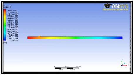
Figure 3. Gage Pressure contours in the 2D pipe for no magnetic field
Figure 4 shows the pressure contours in the domain entirely due to a magnetic field strength of 0.25 T from a current carrying wire at the 3 different locations, i.e. left wire, middle wire and right wire locations (Also see Figure 1). This figure presents a case without any fluid flow and illustrates the nature of the Kelvin body force separately. From analytical theory (presented in the Appendices 1 and 2) the magnetic field surrounding a current carrying wire will form concentric circles of decreasing strength extending from the center of the wire. The effect of this can be observed in the Figure 5 showing the pressure, where isobaric curves are observed to form circles emanating from the location of the wire. These cases serve as a check on the proper operation of the code, especially the UDF. For the case of a wire located upstream of the TR the pressure curves focus upstream, while the same reasoning holds for downstream wires.
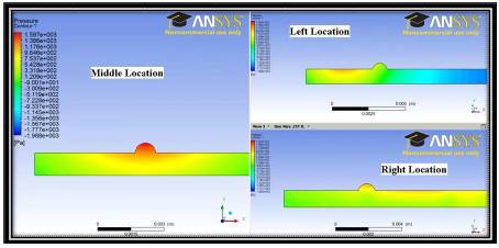
Figure 4. Pressure Contours Entirely Due to the Kelvin Body Force Resulting from Current Carrying Wires at Various Wire Locations in 2D
For the same conditions as illustrated in Figure 4, simulations are now carried out where the magnetic field effects are incorporated into the fluid flow calculation. Figure 5 shows stream lines from three different cases involving magnetic fields from current carrying wires at the three locations. The large regions that the streamlines tend to avoid are regions of recirculation within the flow. This recirculating fluid contains the drug and has the potential to increase magnetic drug transfer due to in the increased retention time of the drug in the target area.
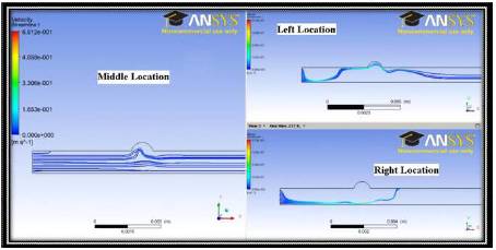
Figure 5. Streamlines for the 2D Case with Magnetic Field Resulting from Current Carrying Wires at Various Wire Locations
Next, Figure 6 presents the pressure contours for two current carrying wires producing a magnetic field of 0.25 T, in the three possible combinations. The linear summation of fields, as suggested by the BiotSavart Law, can be observed.
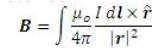
Figure 7 shows the pathlines of particles from the inlet for the same three possible combinations in Figure 6. Again the regions, which tend to repel the streamlines are regions in which the fluid is recirculating. This driven recirculation works to trap the drug molecules in the region of interest longer than if they were to flow along with the bulk of the fluid.

Figure 6. Pressure Contours for the 2D case with Magnetic Field Resulting from Multiple Current Carrying Wires at Various Possible Combinations of Locations
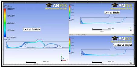
Figure 7. Streamlinesfor the 2D Case with Magnetic Field Resulting from Multiple Current Carrying Wires at Various Possible Combinations of Locations
In a manner similar to the 2D analysis, 3D simulations were performed in the absence of an external magnetic field. Both the pressure and velocity profiles are indicative of traditional pipe flow. Figure 8 shows the pressure contour varies from the inlet to the outlet and the velocity can be seen to form a parabolic profile within the body of the blood vessel. These conditions are representative of laminar fluid flow within a pipe as should be expected from an accurate model of the problem.
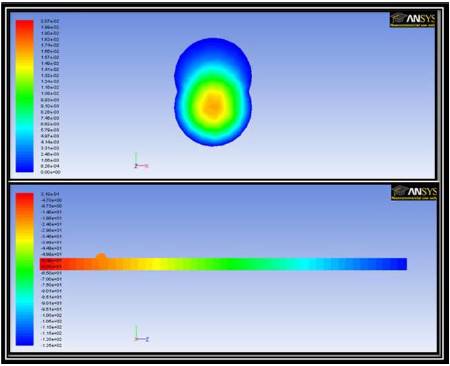
Figure 8. Axial Velocity Contours in a Transverse Cross Sectional Plane in the Targeted Region (top) and Pressure Contours in the Axial Cross Sectional Plane (bottom) for 3d Simulations in the Absence of a Magnetic Field
The field of a current carrying wire has been extended to a 3D model using the same center location. Figure 9, shows the flow solution of a case in which a magnetic field is generated from a wire located directly above the targeted region. The strength of the field is setup so that the field strength at the top of the TR is 1 T. Similar to the 2D case, the pressure contours plotted on the yz-plane passing through the center of the geometry is composed of concentric circles of decreasing strength. For the current case, the velocity contours also shown can be seen to suggest a recirculation in the region of interest (Figure 10).
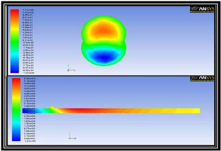
Figure 9. Axial Velocity Contours in a Transverse Cross Sectional Plane in the Targeted Region (top) and Pressure Contours in the Axial Cross Sectional Plane (bottom) for 3d Simulations in the Presence of a Magnetic Field of Strength 1 T
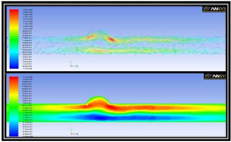
Figure 10. Velocity Vectors in an Axial Cross Sectional Plane Colored by Velocity Magnitude (top) and Axial Velocity Contours in an Axial Cross Sectional Plane (bottom) for 3d Simulations in the Presence of a Magnetic Field of Strength 1 T
The recirculation around the region of interest can be seen more clearly in Figure 10. The velocity vectors clearly show that the fluid is being driven to remain near the region of interest for an extended time. In this case the gradient of the field is sufficient to capture the fluid and promote enhanced drug delivery.
Additional cases show that similar flow is setup from current carrying wires of any strength above some critical strength. It was observed that the magnetic field strength must be reduced to below 0.02 Teslas, as seen in Figure 12 to inhibit the recirculation. In this flow the inertia of the fluid dominates over the effect of the magnetic field. As should be expected trials show that this critical field strength is a function of both blood density as well as velocity. From inspection of the traditional Reynolds number for the fluid flow, the inertia of the fluid depends on density, velocity, and a representative length scale.
For the problem of a blood vessel, the inertia will depend on the blood density, blood velocity, as well as the vessel diameter. Design of a magnetic field to capture the drug must take into account these factors such that the field strength is greater than the critical strength required by the fluid' s inertia.
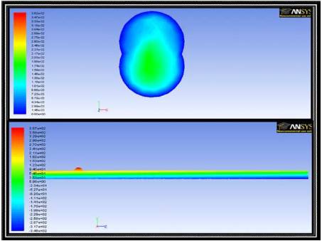
Figure 11. Velocity Vectors in a Transverse Cross Sectional Plane (top) and Pressure Contours in an Axial Cross Sectional Plane (bottom) for 3D Simulations in the Presence of a Magnetic Field with a Uniform Gradient
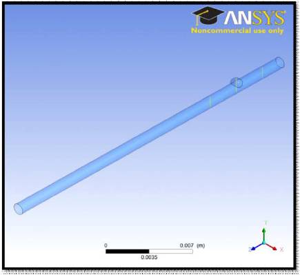
Figure 12. Lines of Reference for Grid-Dependent Studies
In addition to the field of a current carrying wire a uniform gradient field has been generated. Imposed on Figure 11 is a field whose magnitude varies linearly from 0.5 T at the top of the TR to 0.49 T at the bottom of the TR. For this case the effect of the field is similar to that of a “controllable” gravity field. The horizontal pressure bands are similar to the pressure seen from a gravity field. As can be seen in the velocity contours, the fluid is more eccentric from the center of the blood vessel than the benchmark case. The field has pulled additional fluid into the stagnant region of the blood vessel by means of this uniform body force. Although recirculation has not been developed, drug transfer could be enhanced because in a real two-phase scenario the uniform body force would pull only the ferrofluid into the stagnant region. The introduction of the drug into a region, which would have otherwise flown by the TR,could lead to an improved drug transfer.
As demonstrated in both 2D and 3D simulations the effect of various magnetic field orientations and strengths has the potential to dramatically alter the flow characteristics in a blood vessel. Optimization of a drug targeting system has been accomplished through selection of the optimum fluid, EFH3. Additionally, the effect of various fields has been investigated and discussed. The two main mechanisms that could enhance drug transfer are introduction of fluid into a stagnant region with the use of uniform gradients, and recirculation of the fluid with the use of magnetic field from current carrying wires. A comprehensive generalized UDF for the magnetic field effects as the Kelvin body force source term has been designed, incorporated and tested in the context of ANSYS fluid solver.
| Symbol | Units | Description |
| ρ | kg/m^3 | Density |
| ν | m/s | Velocity |
 |
- | Del Operator |
| P | Pa | Pressure |
| F | N | Force |
| µ | kg/(m s) | Dynamic Viscosity |
| µ0 | (T m)/A | Magnetic Permeability of free space |
| g | m/s^2 | Gravitational Force |
| M | A/m | Magnetization |
| H | A/m | Auxiliary Magnetic Field Strength |
| χ | - | Magnetic Susceptibility |
| m | meters | Length |
| x | meters | Cartesian Coordinate System, x direction |
| y | meters | Cartesian Coordinate System, y direction |
| z | meters | Cartesian Coordinate System, z direction |
| r | meters | Radialdistance of point of interest |
| R | meters | Radius of artery |
| Re | - | Reynolds Number |
| d | meters | meters Diameter of artery |
| T | N/(A m) | Tesla |
| A-X | - | Constants used for field strength calculations |
The addition of magnetic affects to the Navier Stokes equation can be accounted for by the Kelvin body force term, shown as the last term in the following equation.
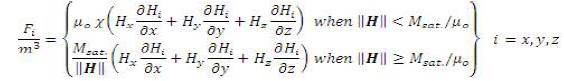
The magnetization in the Kelvin body force term can be summarized as a piecewise equation. When the strength of the magnetizing vector is below the magnetizing saturation the response of the fluid is proportional to the magnetizing field with a coefficient termed magnetic susceptibility. After the strength of the magnetizing field increases above the fluid saturation the fluid's response reaches a plateau.
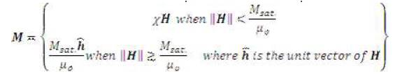
The magnetic body force term can be broken down into appropriate x, y, and z components:
To ensure realistic conditions, the fully developed velocity profile is described as:
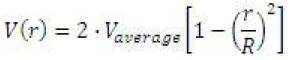
The use of this parabolic velocity profile is accurate for a laminar flow study.
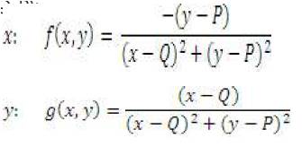
Equation for vector field of current carrying wire, centered at (Q, P):
Equation for vector field of current carrying wire, centered at (Q, P, N), parallel to x-axis
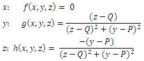
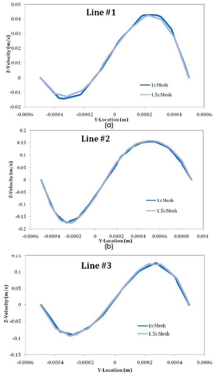
Figure 13. Comparison of velocity profiles across the 3 lines ((a), (b), and (c)) marked in Figure 12, between the coarse and fine meshes