The process by which a flow initially laminar becomes turbulent is called transition. Transition involves a mechanism by which an initially laminar flow changes to laminar-transition state through a series of instabilities and finally becomes turbulent. The location of the onset and extent of transition affects the design and performance of many aerospace devices where the wall heat transfer or wall-shear-stress is of interest. The transition process also influences the separation behavior of boundary layers. An approach to predicting transition is the use of experimental correlations. These correlations (Narshimha, 1989) usually relate the free-stream turbulence intensity, Tu, and the local pressure gradient to the transition momentum thickness Reynolds number (Re_θ).

In present work, the efforts are reported in identifying the transition region. As a first case, two dimensional flow over a flat plate is considered. The simulation is carried out using Large Eddy Simulation (LES) (Eugene, 2006 and Ugo, 1999), because it allows to capture the turbulence behavior till the selected grid size (Δx, Δy, Δz). Since the immediate objective of the experiment is to capture the filtered values only and not the subscale values, the sub-grid scale model ( Smagorinsky, 1963; in our case), is turned 'off' while performing LES. This is achieved by setting the constant Cs to zero. That way only filtered velocities are captured and not the residuals.

In order to identify transition region, cases have been run for two different inlet velocities; U_x = 10 m/s and for U_x = 50 m/s. Air is taken as the flow medium. The variation of vorticity Reynolds number, Reynolds stresses and root mean square (RMS) values of fluctuating velocity component with respect to Reynolds number based on plate length Rex have been studied. This section is immediately followed by some modeling aspects of LES including sub-grid scale modeling. Details of numeric such as equation sets, schemes, computation domain and grid, and boundary condition are briefed in next section. This is followed by results and detailed discussions and finally the whole work are summarized in conclusion.

In LES, the dynamics of the larger-scale motions are computed directly, while the smaller scales sub-grid scales) are modeled separately using a Sub-grid scale model. The four conceptual steps in LES are as follows:

• A filtering operation is defined to decompose velocity U (x,t) into the sum of a filtered (or resolved) component U and a residual (or sub grid scale, SGS) component u′. The filtered velocity field represents the motion of the larger scales.
• The equations for the evolution of the filtered velocity field are derived from the Navier-Stokes equations. These equations are of the standard form with the momentum equation containing the residual-stress tensor that arises from the residual motions.
• Closure is obtained by modeling the residual stress tensor, most simply by an eddy-viscosity model.
• The model filtered equations are solved numerically for U, which provides an approximation to the large-scale motions.

In order to close the equations for the filtered velocity, a model for the anisotropic residual stress tensor is needed. The simplest model is the Smagorinsky model, (Smagorinsky, 1963), which also forms the basis for several other models. The model can be viewed in two parts. As the first point, it is based on Boussinesq eddy viscosity assumption where residual stresses can be modeled as eddy viscosity multiplied by filtered strain rate tensor and is given as (τ_ij = -2ν_t S_ij). The coefficient of proportionality ν_t is the eddy viscosity of the residual motion. Secondly, by analogy with the mixing-Length hypothesis, the eddy viscosity is modeled as

Where S is the filtered rate of strain, l_s is the Smagorinsky length scale, which, through the Smagorinsky coefficient C_s, is taken to be proportional to the square of filter width Δ . For laminar shear flows in which the residual shear stresses are zero, the appropriate value of Smagorinsky coefficient is C_s = 0. A non-zero value of C_s would lead, incorrect residual shear stresses, and thus the skin friction drag (C_f ).

Opensource CFD solver OpenFOAM (OpenFOAM, 2004 and Jasak, 1996) is used to carry out the simulations. The 2-dimensional governing equations (continuity and momentum) are solved for. The standard properties of air are taken, which is assumed to be incompressible. Equations in two spatial dimensions are taken for simplicity and concept building.

The governing equations are discretized on a collocated grid using the finite volume method. Any small scale (smaller than the control volume) motions are filtered out and have to be accounted by a sub grid scale model. For the present study, the sub grid scale model is not employed for first run. In the last case, the authors have employed a varying sub grid scale eddy viscosity (ν_t). The variation is linear between the transition points and constant thereafter. In former case, the ν_t is kept zero throughout.

Time integration is performed with the linearized Euler backward formula. The spatial discretization is second order central differencing which is widely used in LES owing to its non-dissipative and conservative properties. The pressure velocity coupling is done using the PISO algorithm. The system of equations is solved using the preconditioned conjugate gradient (PCG) method with diagonal incomplete Cholesky (DIC) preconditioning for pressure and the preconditioned bi-conjugate gradient (PCiBG) method with diagonal based incomplete LU (DILU) preconditioning for velocity.

The flow domain consists of rectangle [0, 1.6] x [0, 0.5] (Figure 1a). The smallest cell size in the domain has been decided based on Taylors scale as η_t = (√15) C^−1/2 Re_x^−1/2 l_ref. Based on this, 445 x 397 x 1 cells have been taken along the streamwise, wall-normal and spanwise directions respectively. Simple grading of 1.01 has been employed in the wall-normal region which allows the cell size to vary from 0.1 mm to 5 mm. Uniform cell-size of 4 mm is used for the streamwise direction. Since a two dimensional case is being run, single cell is used in the spanwise direction. The computational mesh is shown in Figure 1b.

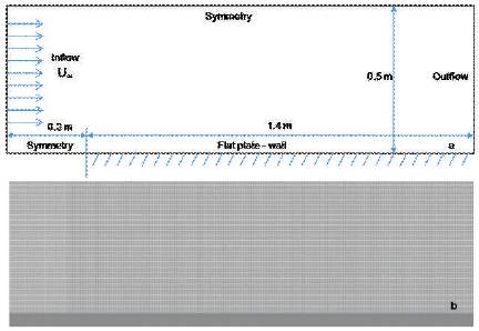
Figure 1. (a) Computational domain with boundary conditions (b) Computational mesh

At inlet, free stream condition is prescribed. Simulations were performed for two inlet velocity values: 10 m/s and 50 m/s. The wall boundary is located at y = 0, x> 0.2. Symmetry condition is imposed at y = 0; 0 < x < 0.2 (Roach et al., 1990). It is assumed that the plate is not there at the inlet. At all other boundaries, zero gradients are prescribed. Free stream pressure is applied at inlet and symmetry boundaries. At outlet, pressure is extrapolated from the interior. The inlet velocity is taken as the initial condition. The laminar flow is allowed to evolve and become unstable leading to transition.

The time step used in the simulations was 10⁻⁵ seconds. The simulation was run for 2.5 x 10⁵ time steps to allow for the transition and the turbulent boundary layer to be established, i.e., the flow has reached a statistically steady state and average results were gathered.

It is expected that the local variables of the boundary layer correlate to the flow transition. Thus, the behavior of vorticity, RMS velocity, and Reynolds stresses are looked into. Their significance on the prediction of transition is explained in the following subsections.

One of the central variables used in identification of onset of transition is the vorticity Reynolds number, Re_ξ

(1)

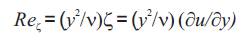
Where 'y' is the distance from the wall. Since the vorticity Reynolds number depends only on density, viscosity, wall distance and the vorticity (or shear strain rate, ξ~), it is a local property and can be easily computed at each grid point in an unstructured, parallel Navier-Stokes code.

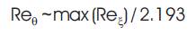
In Figure 2, vorticity Reynolds number is plotted against the wall distance for streamwise locations identified by Re_θ and Re_x. The maximum of the profile is proportional to the momentum thickness based Reynolds number (Re_θ), and thus can be used in the prediction of transition, (Menter et al., 2002-2005) as follows:

(2)

At a particular streamwise location the maximum of Re_ξ (Re_ξmax ) is plotted (Figure 3) against the Reynolds number based on the flat plate length (Re_x). From the plot, it can be seen that there is a sudden jump in the vorticity Reynolds number values at Re_x ~ 3x10⁵. This may be attributed to the increase in the velocity gradient () beyond this critical Reynolds number. This location, which corresponds to momentum thickness Reynolds number Re_θ = 380 can be treated as transition onset. This is consistent with the results obtained by Menter et al. 2002-2005.

A second case (U_x = 50m/s) is run to capture the behavior at higher Reynolds number. From Figure 4, it can be seen that beyond Re_x ∼ 10⁶, the vorticity Reynolds number shoots up again. This location may correspond to the onset of turbulence. However, to identify if these two Rex values are universal, more cases need to be investigated.

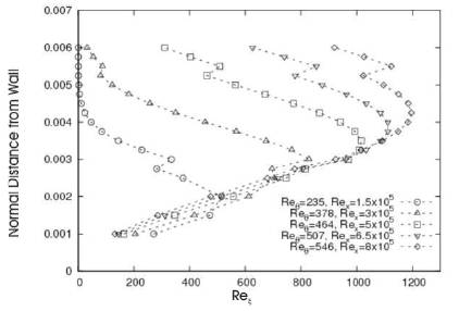
Figure 2. Wall normal distance vs non dimensional time average vorticity (vorticity Reynolds number, Re_ξ)

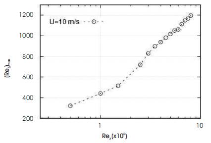
Figure 3. Maximum value of non dimensional average vorticity (Re_ξmax) plotted against Re_ξ

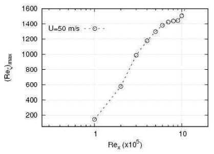
Figure 4. Maximum value of non dimensional average vorticity (Re_ξmax) plotted against Re_x

The variation of Reynolds stresses (u′v′) over the flat plate is also one of the important variables that is considered for transition prediction. To understand the behavior qualitatively, Reynolds stresses were normalized by u_t² (Schlatter et al., 2010), where, u_t = (τ_w/ρ)^0.5, is the friction velocity.

The maximum value at the particular x location is determined. On plotting u′v′_max / u_t² (at a particular streamwise location) against Re_x, it can be seen from Figure 5 and 6 that it is normalized. Reynolds stress starts increasing at Re_x ~ 3x10⁵, indicating transition from laminar regime. Then it again shoots up at Re_x ~ 2x10⁶. This is the transition to turbulence.

The Reynolds number corresponding to the transition onset and turbulence onset is in agreement with the values obtained through vorticity Reynolds number (Re_ξ). Thus, the Reynolds stress can be used to predict both the transition (critical) Reynolds numbers.

Turbulence intensity variation over the flat plate can also be one of the important variables for transition prediction. In a general way, turbulence intensity scales is as

(3)

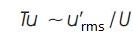
where u′_rms is the root-mean-square of the turbulent velocity fluctuations and U is the mean velocity.

On plotting the maximum of root-mean square of velocity fluctuations at a particular streamwise (x) location versus Re_x, it can be seen (Figure 7, high steepness of the curve) that the turbulence intensity starts increasing near Re_x ∼ 3x10⁵, indicating transition from laminar regime. Then, it again shoots up (Figure 8) around Rex ∼10⁶. This is attributed to the transition to turbulence. The Reynolds number corresponding to the transition onset and turbulence onset is in agreement with the values obtained through vorticity Reynolds number and through Reynolds stresses.

The Smagorinsky constant is zero in the laminar region, linearly varying (from 0 to 0.09) in the transition zone and constant (0.09) in the turbulent one. The skin friction coefficient (C_f ), is plotted (Figure 9) against Re_x and compared with the experimental data published by Roach et al., 1990.

The agreement in the skin friction values is very good in the laminar region. Once the sub-grid model is turned on, the skin friction values increase as expected, due to rise of effective viscosity. The Smagorinsky constant is varied linearly in the transition region, in order to observe the behavior.

The qualitative agreement is good in the transition and turbulent regions. However, there is a significant difference in C_f values. The reasons may be that variations other than linear need to be tried for the Smagorinsky constant. Another point is that a two-dimensional simulation has been carried out, while the turbulence characteristics are three dimensional. Hence, the work has to be extended to three dimensions, for a proper comparison. Further work needs to be carried out in these areas.

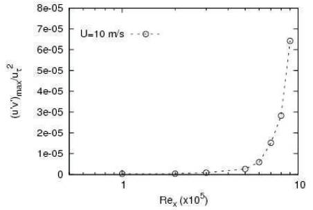
Figure 5. Maximum value of Reynolds stress (u′v′_max/ u_t²) plotted against Re_x

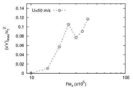
Figure 6. Maximum value of Reynolds stress (u′v′_max/ u_t²) plotted against Re_x

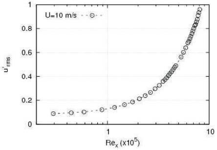
Figure 7. Maximum value of root mean square of velocity fluctuations (u′_rms) at a particular streamwise location plotted against Rex plotted against Re_x

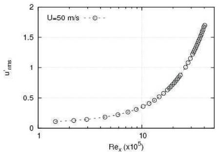
Figure 8. Maximum value of root mean square of velocity fluctuations at a particular streamwise location plotted against Rex plotted against Re_x

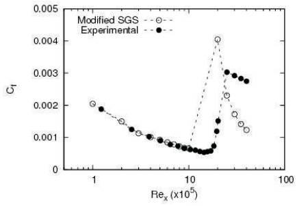
Figure 9. Skin friction coefficient (C_f ) plotted against Re_x

In this work, a simple case of two dimensional flow over a flat plate was considered for transition prediction. Large Eddy Simulation is selected as turbulence model, but without any sub-grid scale eddy viscosity. The behavior of local properties e.g. vorticity Reynolds number, Reynolds stresses and RMS of velocity fluctuations are analyzed near the transition regime. It is observed that onset of transition as well as turbulence can be obtained from the behavior of above local quantities. These plots are all mutually consistent. A linearly varied sub-grid scale eddy viscosity is implemented and the coefficient of skin friction matches well qualitatively with the available experimental data. It differs in transition and turbulent regions where further work is required to develop a numerical model, such that Smagorinsky's constant can be modified based on local vorticity Reynolds number. This work can be extended to three dimensional flow over a flat plate as well as for a more complex geometry such as airfoils. Then, it can be established whether the methods used for transition prediction are universal or not. The variation of the Smagorinsky constant in the transition region can also be looked into.

Authors are thankful to Dr. Dhananjay Brahme and Mr. Kishor Nikam from Computational Research Laboratories (CRL) for the initiation of this work. Also authors express their profound gratitude to CRL for providing the supercomputing facility, Eka.

Instantaneous field variables were stored during the simulations for the purpose of analysis. At the end of every time step, the code was modified in such a way that the velocity field was written to a file using an in-built function within OpenFOAM. Also to obtain vorticity values at each time step, curl of velocity was calculated at end of every PISO loop as vorticity = curl(U). The corresponding vectorfield (vorticity) was declared in the create Fields. H header file, which is modified as follows:

volVectorField vorticity

IOobject

(

”vorticity”,

runTime.timeName(),

mesh,

IOobject MUST READ,

IOobject::AUTO WRITE

),

mesh

);

IOobject::MUST READ indicates that the vorticity field has to be initialized at time t=0.

IOobject::AUTO WRITE indicates that the vorticity values will be written to a specific output file. This header file is included at the beginning of the solver code (e.g. pisoFoam.C). Finally, the code was compiled and run on the case. Similarly, vorticity Reynolds number was computed at each time step with the following modifications at the end of the PISO loop within pisoFoam.C file:

patchDist y(mesh, true);

Info<< ”Writing wall distance to field ”

<< y.name() << nl << endl;

y.write()

Retheta = y*y*vorticity/1.7e-05;

Retheta.write();

The function, patchDist, returns distance from the wall for each cell within the domain. Another function, write(), prints the value to the screen at every time step. Just like the previous case, the variable Retheta has to be declared in the create Fields. H header file.