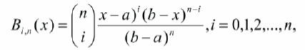
where,
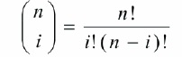
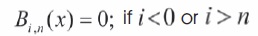
is the binomial coefficient or Bezier coefficient. For convenience, set
Polynomials in Bernstein form were first used by Bernstein (Bernšteın, 1912) in a constructive proof of the Stone-Weierstrass approximation theorem. With the advent of computer graphics, Bernstein polynomials restricted to the interval x ∊ [0, 1] became important in the form of Bezier curves.
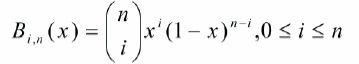
1.2 Definition 2
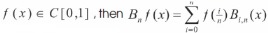
The Bernstein basis polynomials of degree n on [0, 1] are defined by,
and the nth degree Bernstein polynomial of the function f (x) on [0, 1] is expressed as,
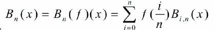
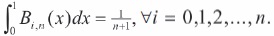
1.3 Properties of Bernstein Polynomials
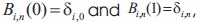 where is the Kronecker delta function.
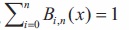
- The Bernstein basis polynomials form a partition of unity i.e.,
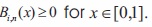
- The Bernstein basis polynomials are all non-negative i.e.,
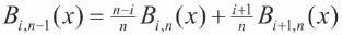
- Any of the lower-degree Bernstein polynomials (degree < n) can be expressed as linear combination of Bernstein polynomials of degree n.
- Let
 converges to f(x) uniformly on [0, 1] as n⟶α
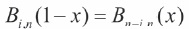
- For a given
1.4 Theorem 1 - Bernstein Approximation Theorem (Lorentz, 1953)
A bounded function f(x) on [0, 1] holds the relation,
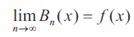
at each point of continuity x of f; and the relation holds uniformly on [0, 1], if f(x) is continuous on this interval.
2. Main Results
In most of the recent works (Ahmed, 2014; Dascioglu & Isler, 2013; Bhatti & Bracken, 2007), solutions to the differential equations have been obtained using Bernstein polynomial basis along with Galerkin method or Collocation method or Dual basis method respectively. Pandey and Kumar (2012) solved linear and nonlinear homogeneous differential equations using Bernstein polynomial basis with Tau method. With this motivation, in this paper we discuss the solutions of higher-order linear differential equation, Bessel and second order parabolic equations using Bernstein basis polynomials with Tau method. In this paper Bernstein Tau method is proposed and by using the theorem 1, an approximate solution of differential equations in terms of truncated Bernstein series is assumed to be of the form.
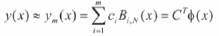
Here  and ym is the mth degree Berstein approximate solution of y.
2.1 Fundamental matrix Relations
We know that,
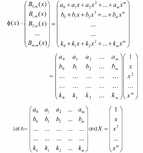
Then  which implies
Further, 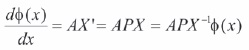
where,
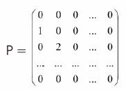
The first operational matrix of differentiation is D(1) = APA-1 . That is,
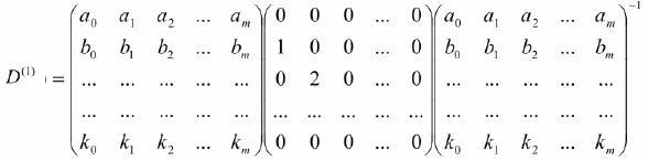
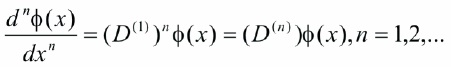
It can be generalized as,
2.2 Bernstein Tau Method
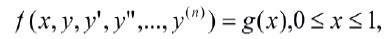
Now consider the nth order nonhomogeneous linear differential equation of the form,
satisfying initial conditions,
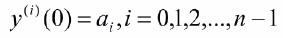
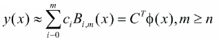
Using Equation (6), y(x) can be approximated as,
Here the unknown coefficients ci, i = 0, 1, 2, ..., m are obtained by using Bernstein Tau method. In view of Equation (8) and (11), Equation (9) can be written as,

The initial conditions in Equation (10) are transformed as,

Define the residual R (x) for equation (12) as,

The unknown coefficients ci are calculated using Tau method (Pandey & Kumar, 2012), that is,

Which yields m - n linear equations corresponding to the values of i. Equations (13) and (15) constitute set of m + 1 linear equations. The unknown coefficients c0 , c1 , ..., cm are obtained by solving these m + 1 linear equations and hence the Bernstein approximate solution ym (x) is obtained by submitting unknown coefficients ci in equation (6).
The values of the residual function at xa ∈ [0, 1], q = 0, 1, 2, ...

determine the accuracy of the truncated Bernstein series solution equation (6), (9) and (10). Evidently ǀRm (xq)ǀ ≤ 10-ki , where ki is a positive integer and i = 0, 1, 2, 3, ... . If k = max {k|i = 0, 1, 2, 3, ...} and 10-k is the prescribed error limit, then the truncation limit m is increased until ǀRm (xq)ǀ at each of the points becomes smaller than the prescribed error limit.
3. Test Problems and Numerical Results
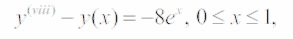
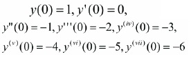
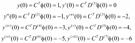
Example 1. Consider the eighth-order linear differential Equation.
satisfying initial conditions,
The above problem has been solved by Mestrovic (2007) using modified decomposition method. Now, we apply Bernstein basis polynomials with Tau method to solve the problem. The exact solution of Equation (16) is y(x) = (1-x)ex.
Using Bernstein basis polynomials, y(x) can be approximated as,
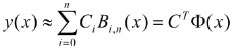
where C = [c1, c2, ...cn]T contains unknown coefficients of the expansion and 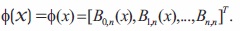
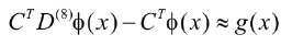
Using Bernstein operational matrix of differentiation, Equation (16) can be written as,
The residual Rn(x) for Equation (18) can be written as,

Applying Tau method (Pandey & Kumar, 2012), Equation (18) can be converted into n-8 linear Equations with the condition.

The initial conditions are given by,
Equation (19) and (20) generate n + 1 set of linear equations. These equations are solved for unknown coefficients ci and hence the Bernstein approximate solution ym (x) is obtained.
The comparison of the absolute errors is given in Table 1 and the comparison of results in Table 1 shows the superiority of the present method over the method of Meštrović (2007) for n = 8. Figure 1 shows that the approximate solution in the present method almost coincide with the exact solution. The absolute errors are shown graphically in Figure 2.
Example 2. Consider the Bessel differential Equation of order zero.
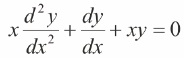
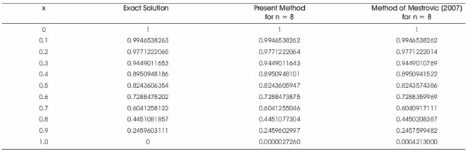
Table 1. Comparison of Numerical Results of Example 1 for n = 8
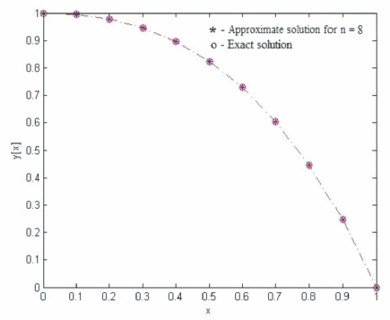
Figure 1. The Exact and Approximate Solutions of Example 1 for n=8
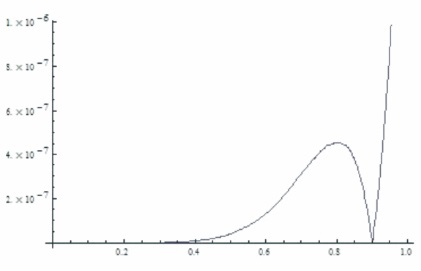
Figure 2. Comparison of Absolute Errors of Example 1
With the initial conditions,
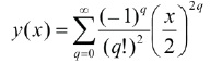
It has been solved by using Chebyshev wavelets and the results were compared with the method of Razzaghi and Yousefi (2000) in Babolian and Fattahzadeh (2007). Now, we apply Bernstein basis polynomials with Tau method to solve the problem. The exact solution of equation (21) is,
The comparison of the absolute errors is given in Table 2 and the comparison of results in Table 2 shows the superiority of the present method over the methods of Babolian and Fattahzadeh (2007) and Razzaghi and Yousefi (2000) for n = 5. Figure 3 shows that the approximate solution in the present method almost coincide with the exact solution. The comparison of absolute errors for n=3, 4, 5, and 10 is given in Table 3 and these values assert that the convergence of the method become faster as degree of Bernstein polynomials is increased.
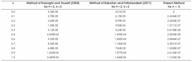
Table 2. Comparison of Numerical Results of Example 2 for n = 5
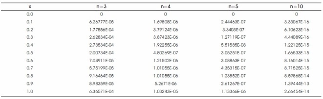
Table 3. Comparison of Absolute Errors of Example 2
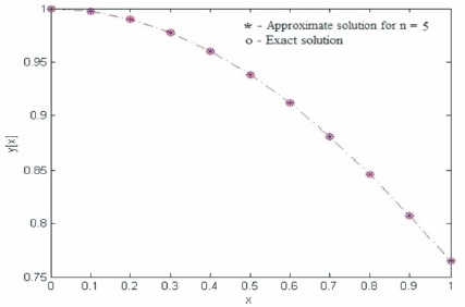
Figure 3. The Exact and Approximate Solutions of Example 2 for n=5
4. Solution of Second Order Parabolic Differential Equation
This section presents an algorithm for approximating solutions to second order parabolic linear differential Equation.
Consider the heat transfer Equation,
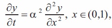
subject to the Initial-boundary conditions,
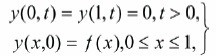
where f(x) is given source function. Ahmed (2014) solved the above problem using orthonormal relation of Bernstein polynomials with its dual basis.
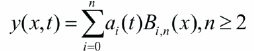
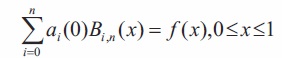
In this paper, we apply Bernstein polynomial basis with Tau method to solve the problem. An approximation to the solution of equation (23) in Bernstein basis polynomials is assumed to be of the form,
In view of Equation (25), Equation (23) and (24) take the form,
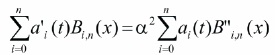
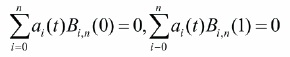
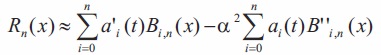
The boundary conditions in equation (27) determined coefficients a0(t) = 0 and an(t) = 0. The residual Rn(x) for equation (23) can be written as,
Applying Tau method (Pandey & Kumar, 2012), equation (26) can be converted to n-2 linear equations with the condition,

The system of equations can be reduced to the following matrix differential form,
where  and A is a square matrix of order n - 1. Thus, the coefficients
  are obtained by solving the differential equation (31). An analytical solution of equation (31) is given by,
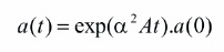
The coefficients a(0) = [a1(0), a2(0), ..., an−1(0)] involving in Equation (28) are obtained by Tau method (Pandey & Kumar, 2012). In order to get a(t) substitute a(0) into Equation (32). Hence the Bernstein approximation solution of y(x, t) is obtained. −π2t The exact solution of Equation (23) for α = 1, f (x) = sin(πx) has the form y(x, t) = e-π2t sin(πx). The comparison of the absolute errors is given in Table 4 and the comparison of results in Table 4 shows efficiency of the present method over the method of Ahmed (2014) for n = 5.
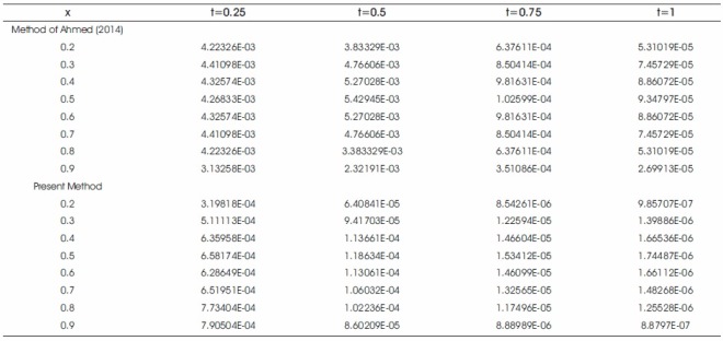
Table 4. Comparison of the Absolute Errors Obtained by Present Method with Method of Ahmed (2014) for n = 5
Conclusion
In this article, higher-order linear differential equations and second order parabolic differential equations are solved by using Bernstein basis polynomials and Tau method. In each of the three problems, the approximate solutions obtained by the present method are compared with the exact solutions, and the numerical results of other methods. The present method shows its efficiency and simplicity over other existing methods. All of these calculations and graphs are done by using Mathematica (Wolfram, 2004).
Acknowledgements
The authors acknowledge the reviewers for their excellent comments and elevating the quality of the article.