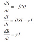
with the initial population strength S(0)= S0, I(0) =I0, R(0)=R0
The Model (1) was subjected to many transformations and finally changed into SIRS models. In this work, we consider nonlinear Incidence rate  with time delay. We investigate the stability analysis SIRS model. The model possess two equilibrium points. The endemic equilibrium point is locally asymptotically stable. We also derived the sufficient conditions for existences of Hopf bifurcation and the results are supported by numerical simulation.
1. Literature Review
The non-linear dynamics was studied by L. S. Chen and Chen. Anderson and May (1979) illustrated biological and infectious diseases models. In the epidemic models, total population is divided into three classes (S, I, R). Let S (t) represent susceptible population, I (t) represents infected population, and R (t) represents removable population. Mena-Lorca and Hethcote (1992) discussed the SIR epidemic model. SIR epidemic models with distributed delay and time lag was discussed by Beretta (1995, 2001), respectively.
Incidence rate plays a significant role in epidemic modelling. Many authors suggest two incidence rates, i.e bilinear incidence rate βSI and standard incidence rate βSI/N in epidemic models. The standard incidence rate may be good approximation if the available frequency of population (N) is large enough. In fact, the infection risk will be influenced by the ability per contact rate of infection probability. This factor plays a key role in spreading of infection. Capasso and Serio (1978) introduced a saturated incidence rate  into epidemic models. Here βSI measures the transmission rate of the disease and
  measures the inhibition effect from susceptible to infective population. Here f(I) tends to a saturation level due to crowding of infective population (I close to large values). This incidence rate seems more reliable than the bilinear incidence rate βSI. Authors (Kermack & McKendrick,1927; Kumar et al., n. d.; Li & Wang, 2009; Liu et al., 1987; Ruan & Wang, 2003) dealt with SIR epidemic models with this incidence rate.
In this work, we proposed SIRS model with the incidence rate and studied the dynamics of the SIRS model with susceptible (S), infective (I), recovery (R) population and incidence rate . The governing equations of the system are as follows. Time delays play a significant role in stability analysis. The delay arguments in SIRS is dealt by authors (Pang & Chen, 2007; Wen & Yang, 2007). Xu & Ma (2008) discussed the stability analysis of SIRS model with non-linear incidence rate and derived the sufficient condition of global stability analysis of the endemic equilibrium point.
2. Mathematical Model
The governing equations of the system are as follows
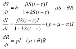
with the following notations
b is the recruitment rate of the population.
β is the transmission rate.
μ is the natural death rate of the populations.
θ is the rate at which recovered individuals lose immunity and return to the susceptible class.
p is the recovery rate of the infective individuals,
α is the death rate due to disease.
k is the parameter which measures the effect of physiological or other mechanisms.
The basic reproduction rate of the System (2) is given by 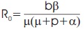
If R 0>1 , the endemic equilibrium point exist and if R0<1 the system has no feasible solution.
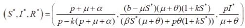
3. Steady State Points
The System (2) has two steady (Equilibrium) states given by,
Disease free equilibrium point E1 is

Endemic equilibrium point (E2) is,
4. Local Stability of Analysis at Endemic Equilibrium Point
The variational matrix for the System (2) is given by,
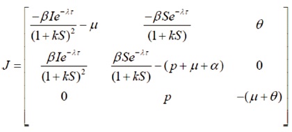
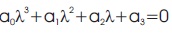
with the characteristic equation
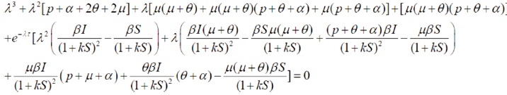

We need to find the condition for existence of negative real roots.
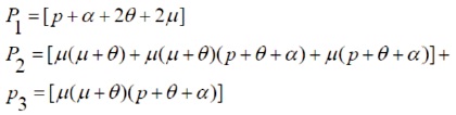
Case (I): For τ = 0, Equation (5) becomes
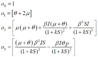
Where,
Calculate the following determinates
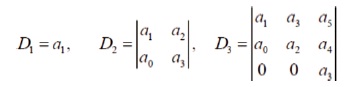
D1 =[θ+2μ], which is a positive value
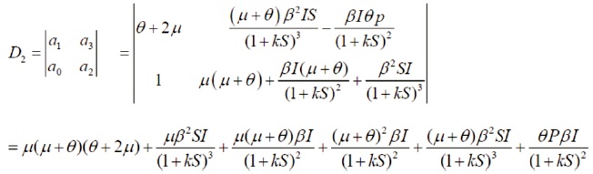
D2 is also a positive value
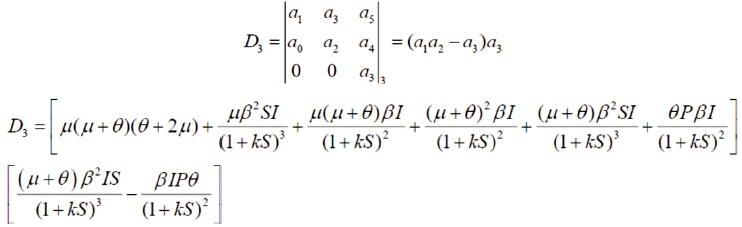
D3 is also a positive value if 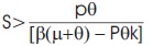
Using Routh –Hurwitz criteria all the three determinates are positive. Hence the system is asymptotically stable if
Therefore, endemic equilibrium E(S*, I*, R*) is locally asymptotically stable.
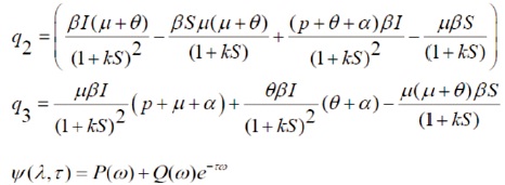
Case (ii) for τ > 0: Suppose there is positive τ0 such that the Equation (5) has pair of purely imaginary root ,can be taken as iω, ω>0 then separating real and imaginary part in Equation (5) after putting λ =iω, ω>0 we have,
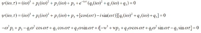


(9)2 + (10)2 ⇒
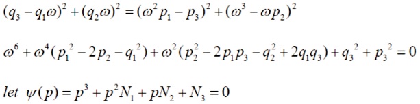
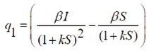
Where,
If we assume that N1>0, N2>0, N3>0 then have no positive real roots.
N1=p12-2p1–q12 N2 =p22 -2p1p2–q22 + 2q1q3 N3 =q33+p33
Thus if N1>0, N2>0, N3>0 then there is no ω such that iω is an Eigen value of the characteristic equation of Ψ(λ, τ)=0
If λ will never be a purely imaginary root of equation Ψ(λ,τ)=0,then the real parts of all Eigen values of Ψ(λ,τ)=0 are negative for all τ≥0 summarizing. From the above analysis, we have the following theorem.
Theorem 1. The endemic equilibrium E, is locally asymptotically stable for all τ, if the following condition hold.
- (p1 +q1 )>0, (p2 +q2 )>0, (p3 +q3)>0
- N1>0, N2>0, N3>0
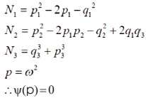
Now if any one of N1, N2, N3 is negative then Model (1) has positive root ω0
Eliminating cos ωλ from Equations (2) & (3)
where k=0,1,2,3..................
By continuity, the real part of λ(t) becomes positive when τ>τ0 and the steady state becomes unstable and moreover, a hopf bifurcation happens when τ passes through the critical value.
4.1 Hopf Bifurcation
Theorem 2: If R0 > 1 there exist a positive τ0 such that the following results hold,
- If 0< τ< τ0, the System of Equations (2) has a endemic equilibrium point E2, is which locally asymptotically stable.
- •The System (2) exhibits a Hopf bifurcation if τ>τ0.
Proof: Hopf bifurcation occurs when the real part of λ(t) becomes positive when τ>τ0 and the steady state becomes unstable, and moreover, τ passes through the critical value τ0.
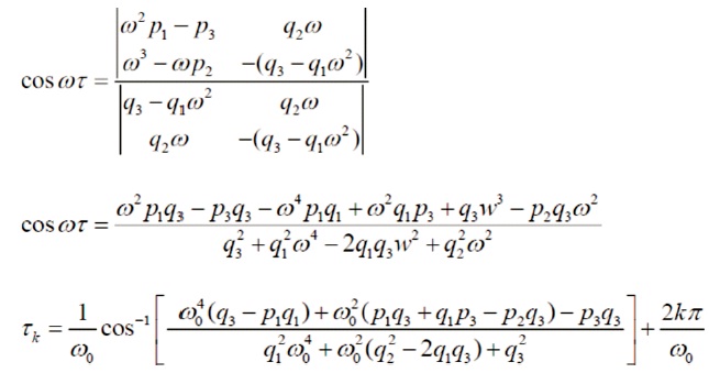
Now differentiating Equation (5) w .r t. τ, we obtain
Under the condition that p12-2p1-q12>0 & p22-2p1p2-q22+2q1q3>0
We have 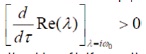
Therefore the Hopf bifurcation occurs at τ = τ0
5. Numerical Example
We study the hopf bifurcations for the System (2) with the tolerance parameter (τ). For the system of equations, the parameters are identified as shown in the following examples. For different values of τ, the graphs are shown below (Figure 1-8).
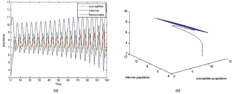
Figure 1. Unstable Variations of System (2) when τ =0.4601
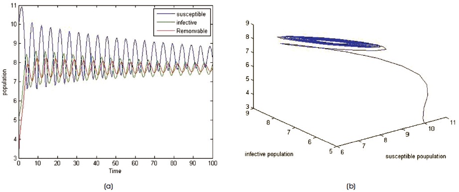
Figure 2. Unstable Variations of System (2) when τ =0.4461
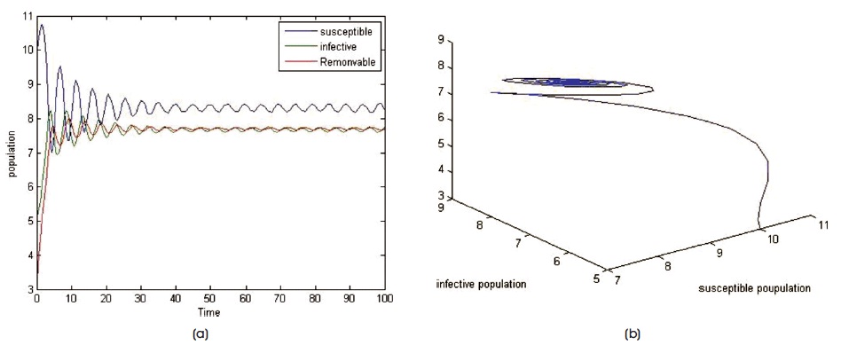
Figure 3. Stable Variations of System (2) when τ =0.3961
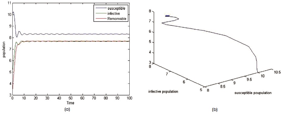
Figure 4. Stable Variations of System (2) when τ =0.1961
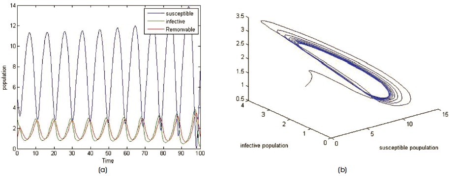
Figure 5. Unstable Variations of System (2) when τ=1.1019
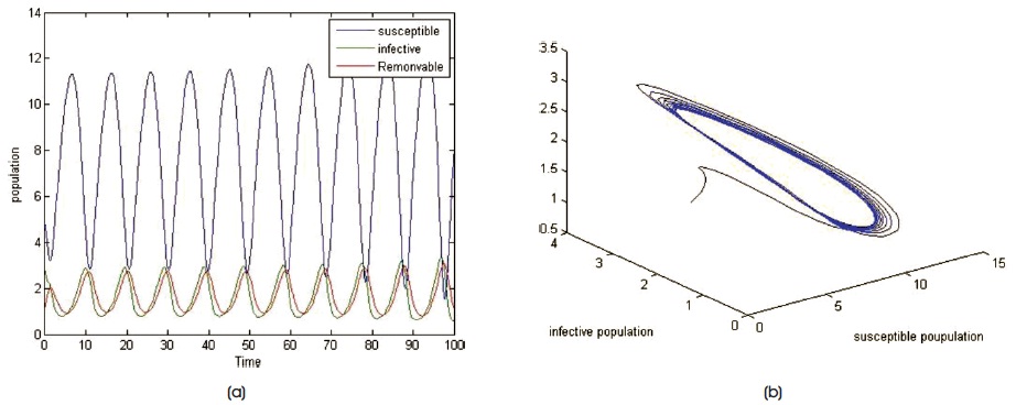
Figure 6. Unstable Variations of System (2) when τ =1.0991
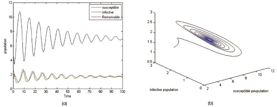
Figure 7. Stable Variations of System (2) when τ =0.8991
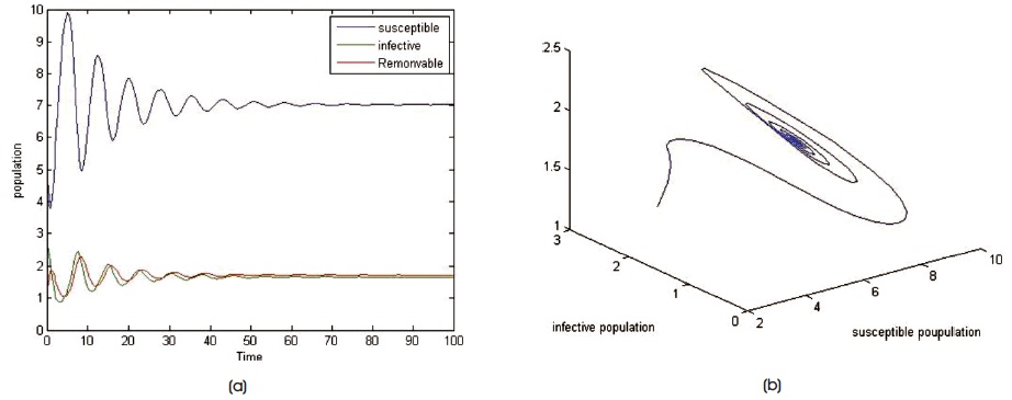
Figure 8. Stable Variations of System (2) when τ =0.6211
Table 1 exhibits the Critical Positive Value (τ0) of both example 1 and 2.

Table 1. Critical Positive Value (τ0)
6. Results and Discussion
Numerical simulation is carried out in support of bifurcation analysis. We choose two set of parametric values and identified the critical bifurcation parameter (τ0). The critical parameter (τ0) for each example is given as follows.
In Example 1 we choose a set of parametric values of the System (2) and simulate using MATLAB. The solution curves are bounded upo to τ0 = 0.44 , later the trajectories are unbounded that leads to unstable system . Hence Hopf bifurcation exist for τ0 = 0.46.
Similarly we choose another set of parametric values and identified that the critical valueτ0 = 0.9 makes system stable to unstable which caused Hopf bifurcation.
Hence the system exhibits Hopf bifurcation and the stability analysis depends on critical positive value (τ0).
Conclusion
We consider an SIRS epidemic model with delay and incidence rate  System admits two equilibrium points. The system is asymptotically stable at endemic equilibrium point if
 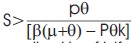 . Sufficient conditions are derived for the existence of Hopf bifurcation. The critical value τ0 is identified where the Hopf bifurcation took place. The sufficient conditions for Hopf bifurcation are derived. The Hopf bifurcation exist if p12-2p1-q12>0 & p22-2p1p2-q22 + 2q1q3>0 where the values of p1, p2, p3 and q1, q2, q3 are given by Equation (6).