The lossy transmission lines terminated by various circuits have many applications to radio engineering devices, in particular to antenna feeder devices, various type waveguides and so on. Many cases are considered in (De Broglie, 1941; Holt, 1963; Jordan & Balmain, 1968; Ramo, Whinnery, & Van Duzer, 1994; Chua, Desoer, & Kuh, 1987; Chua & Lin, 1980; Rosenstark, 1994; Maas, 2003; Misra, 2004; Miamo & Maffucci, 2001; Martin, 2015; Singh, 2013; Makwana & Bhalja, 2016; Ruikar, 2016; Kalaga & Yenumula, 2016; Patil & Behere, 2019; Kapoor, 2019; Dinakaran, 2015; Gaurav & Chauhan, 2016; Raghuwanshi, Kumar, & Pandey, 2011; Sharma, Sandhu, & Sharma, 2018). Many circuits in radio engineering contain as a component the basic loads connected in series. In (Angelov & Hristov, 2011), they have investigated a lossy transmission line terminated by in series connected RLC- elements. We have applied the method from (Angelov, 2013) for solving the mixed problem for hyperbolic transmission line system. Conditions are obtained guaranteeing distortionless propagation of TEM waves. The essential role plays the Heaviside's condition h=(R/L)-(G/C)=0, where R, L, C, G are the specific parameters of the lossy transmission line. It is known, however, that over time, the values of these parameters change and the Heaviside's condition is violated. That is why, the main purpose of the present paper is to investigate the same problem from (Angelov & Hristov, 2011), but without the Heaviside's condition. This does not allow the approach developed in (Angelov, 2013) to be applied. We extend the A. D. Myshkis method, cf. (Angelov, 2015; 2016) to reduce the mixed problem for hyperbolic transmission line system to an operator form and then apply the fixed point technique. We show explicitly that we have to short the line length to obtain a unique solution. On the rest part of the line, the uniqueness of the solution vanishes.

The paper consists of five sections. In Section 1, the boundary conditions are derived using the Kirchhoff's law and formulate the mixed problem for transmission line equations. In Section 2, the hyperbolic system is reduced to a diagonal form. In Section 3, the nonlinearities of the loads are analyzed and an operator formulation of the mixed problem is given. In Section 4, an existence-uniqueness theorem is proved, but not on the whole line. The authors have used the fixed point method. In Section 5, the authors demonstrate conditions of the existence-uniqueness theorem using specific numerical data. And finally, the conclusion is given at the end.

In accordance with the Kirchhoff's law (cf. Figure 1) for the left end of the line we have,

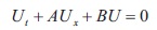
For the voltage at the right end u_{right end} we obtain:

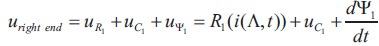
We use usually accepted denotations R₁(i), C₁(i), L₁(i), for the characteristics of the nonlinear loads.

To calculate the voltage of the condenser C₁, we proceed from the relation (assuming u_C1(0)=0):

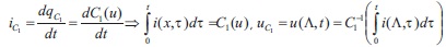
In order to calculate the voltage of the inductor L₁, we use the relation:

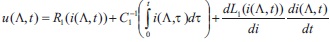
For the right end, that is x = ⋀, we obtain

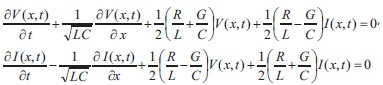
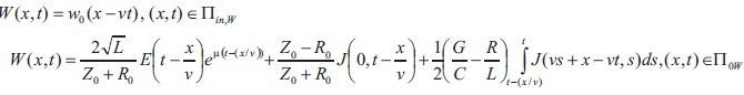
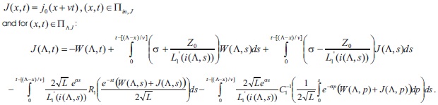
We proceed from the lossy transmission line system (or generalized telegrapher equations) of equations

(1)

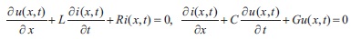
where the unknown functions are voltage u(x, t) and current i(x, t) along the line, L is per unit-length inductance, C - per unitlength capacitance, R - per unit-length resistance, G - per unit-length conductance, ⋀ - the length of the transmission line, and ν=1/√LC - the speed of propagation of the TEM-waves. This system is of hyperbolic type and we can formulate a mixed problem: to find a solution (u(x, t), i(x, t)) for (x, t) ϵ π = {(x, t) ϵ R² : 0 ≤ x ≤ ⋀, t ≥ 0}, satisfying the initial conditions u(x, 0)= u₀(x), i(x, 0) = i₀(x) for x ϵ [0, L], where u₀(x), i₀(x) are prescribed functions. The boundary conditions were derived on the basis of the Kirchhoff's laws in Figure 1.

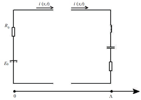
Figure 1. Lossy Transmission Line Terminated by in Series Connected RLC-Elements

The boundary condition for x=0 is

and for x=⋀

To reduce the mixed problem to an initial value problem on the boundary we follow (Angelov, 2015). Rewrite equation (1) in a matrix form:

(2)

where

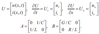
To transform the matrix in a diagonal form we form, the matrix H by eigenvectors, 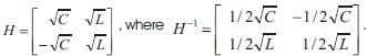, where .It is known that .

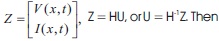Then we introduce new variables Then

(3)

and

(4)

Substituting U = H^-1Z in (2) we obtain,

(5)

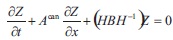
or

(6)

Here we emphasize that the Heaviside condition is not fulfilled, that is, Introducing denotation we make one more substitution 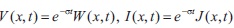and then equation (6) becomes

(7)

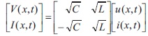
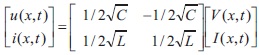
Since we can't apply the method from (Angelov, 2015). By using the transformation formula,

and their inverse ones

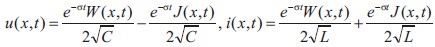
we obtain the initial conditions and respect to the new variables W(x, t) and J(x, t):

Assumptions (L): We assume that the I-L characteristic of the inductive element satisfies conditions:

We need the estimate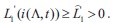

Assumptions ( C): The capacitive element has a characteristic , where are prescribed positive constants.

In view of the obvious singularity of the function C₁(u) we consider C₁(u) for

Since 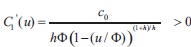and 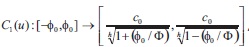the inverse function of C₁(u) does exist and 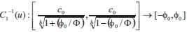Besides since 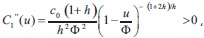, the C1(u) is min 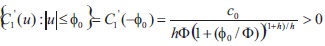We have also 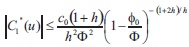and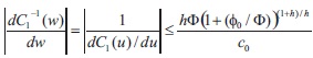

Assumptions (R): and . We assume that

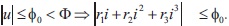
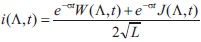
With respect to the new variable (in view of we have to solve the following mixed problem (MP): to find a solution with boundary conditions

where

Following (Angelov, 2016; Angelov & Hristov, 2016) we consider the Cauchy problem for the characteristics:

(8)

(9)

Functions λ_w(x,t)= ν>0 and λ_J(x,t)= -ν<0are continuous ones and imply a uniqueness to the left from t of the solution of and respectively of

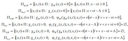
Denote by X_w(x, t), the smallest value of τ such that the solution 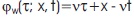of equation (8) still belongs to P and by c(x,t) - the respective value of t for the solution ( ; x, t)=- -vτx - vt of equation (9). If (x, t)>0 then φ_J(X_J(x, t); x,t)=0 or φ_J(X_J(x, t); x,t)= , and respectively if (x, t)>0 then φ_J(X_J(x, t); x,t)=0 or φ_J(X_J(x, t); x,t)= ⋀. In our case

Remark 1: We notice that

It is easy to see that

Introduce the sets

Prior to present the mixed problem in operator form we introduce

and

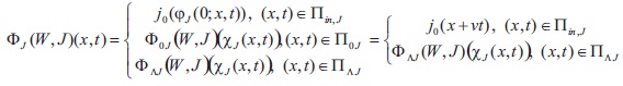
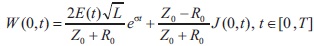
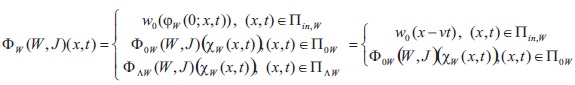
where φ_0w and φ_⋀J respectively are defined by the right-hand sides of corresponding boundary conditions. So we assign to the above mixed problem the following system of operator equations

Introduce the function sets:

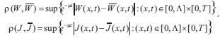
where W_o, J_o and μ>σ are positive constants. It is easy to verify that the set M_w x M_J turns out into a complete metric space with respect to the metric:

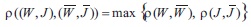
where

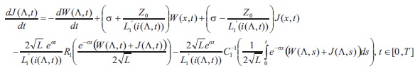
Now we define an operator by the formulas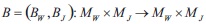

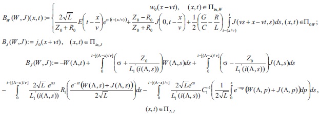
The fixed point (W, J) of the operator B:B_w (W,J);J=B_J(W,J) we call a generalized solution of the mixed problem (MP). In this manner we avoid the conformity condition (Angelov, 2015).

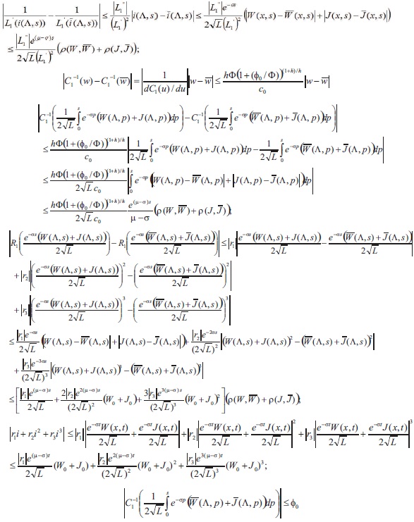
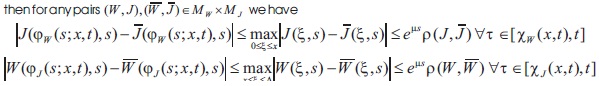
Lemma 1: The following estimates are valid:

Theorem 1: Let the following conditions be fulfilled:

1) E₀ is continuous on with W₀₀, J₀₀ and E₀₀ sufficiently small.

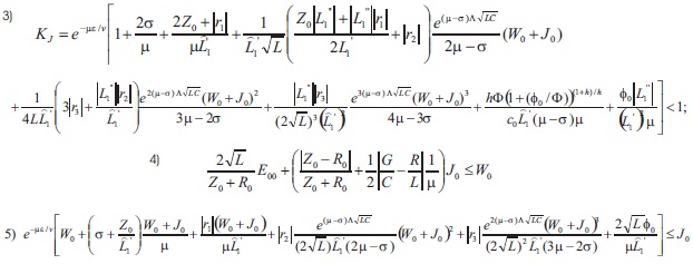
For sufficiently large μ> σ > 0 and some ε ϵ(0,⋀), the following inequalities are fulfilled:

Then there exists a unique generalized solution of equation (3) for

Remark 1: It is easy to see that

Proof: We have to show that the operator B is a contractive one. Indeed, since

and we obtain

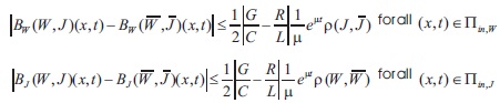
Moreover, if (x,t)ϵπ_ow, then

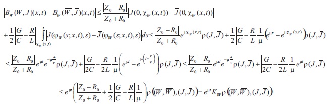
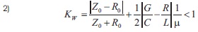
where , which implies

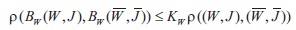
It is easy to see that K_w< 1.

Further on we take into account that for sufficiently large 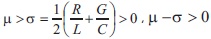is sufficiently large too. Then for (x,t) ϵ π_in,J

which implies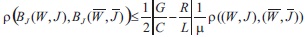

For (x,t) ϵ π_⋀J we estimate the difference below for maximal value of

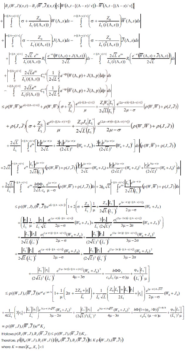
We show that B maps M_w x M_J into itself. Indeed, with the corresponding conformity conditions, all operator functions are continuous ones and: if (x,t) ϵ π_ow, then

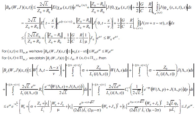
Therefore, the operator B has a unique fixed point which is a generalized solution of (MP);

Theorem 1 is thus proved.

Here we collect all inequalities guaranteeing the existence-uniqueness result,

Let the transmission line be such that L=2.10^-8 H/m ; C=8.10^-12 F/m; R=0,4W/m; G=8 S/m;

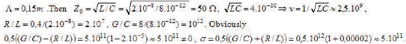
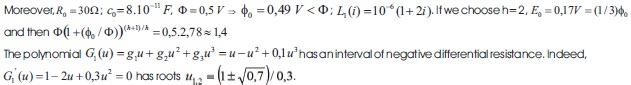
We take the I-L characteristic of the inductive element to be:

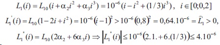
Let us choose i₀ = J₀.Then

Assumptions (R): We assume that

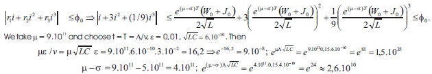
Further on we assume W₀=J₀=E₀₀ and the inequalities from Theorem 1 become:

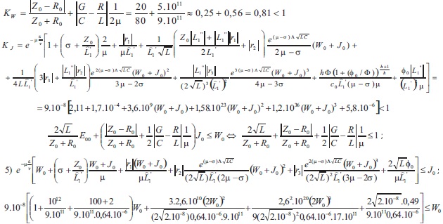
for sufficiently small W₀ and W00.

 It is easy to see that Theorem 1 guarantees an existence of a generalized solution of the mixed problem. For the whole interval [0, L] the solution can be extended as in (Angelov, 2016).

The systems of differential equations arising in electrical engineering are most often solved by numerical methods, the most common of which is Finite Difference Time Domain method (Chan, 2006). Here the author proposes a sequence of successive approximations tending to the solution with respect to the metric introduced. The iterations can be obtained from the operator equations as follows:

beginning with some initial approximation (W⁽⁰⁾, J⁽⁰⁾). It is known that the rate of convergence is

where the contraction constant depends on the parameters of the physical problem. The first approximation can be chosen in various ways, for instance as a solution of the linearized equations of the system. The solution on the interval [L-e, L] can be obtained as in (Angelov, 2016).