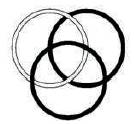
Figure 1. Borromean rings
In this article, the author discussed the concept of Mathematical Knot Theory and Knot Polynomial. And finally the author collects different knots which are used in the mathematical knot theory. In Mathematics, a knot is an embedding of a circle in 3-dimensional Euclidean space, R3, considered up to continuous deformations (isotopies). A crucial difference between the standard mathematical and conventional notions of a knot is that, mathematical knots are closed-there are no ends to tie or untie on a mathematical knot. Physical properties such as friction and thickness also do not apply, although there are mathematical definitions of a knot that take such properties into account. The term knot is also applied to embeddings of Sj in Sn , especially in the case j= n-2. The branch of Mathematics that studies about knot is known as Knot Theory.
Creating a knot is easy. Begin with a one-dimensional line segment, wrap it around itself arbitrarily, and then fuse its two free ends together to form a closed loop. One of the biggest unresolved problems in knot theory is to describe the different ways in which this may be done, or conversely to decide whether two such embeddings are different or the same. Before one can do this, they must decide what it means for embeddings to be "the same". Two embeddings of a loop are considered to be the same if one can get from one to the other by a series of slides and distortions of the string which do not tear it, and do not pass one segment of string through another. If no such sequence of moves exists, the embeddings are different knots. A useful way to visualize knots and the allowed moves on them is to project the knot onto a plane - think of the knot casting a shadow on the wall. Now he can draw and manipulate pictures, instead of having to think in 3D. However, there is one more thing to be done - at each crossing it must indicate which section is "over" and which is "under". This is to prevent us from pushing one piece of string through another, which is against the rules. To avoid ambiguity, one must avoid having three arcs cross at the same crossing and also having two arcs meet without actually crossing (it can be said that the knot is in general position with respect to the plane). Fortunately, a small perturbation in either the original knot or the position of the plane is all that is needed to ensure this.
In topology, knot theory is the study of mathematical knots. While inspired by knots which appear in daily life in shoelaces and rope, a mathematician's knot differs in that the ends are joined together so that it cannot be undone. In mathematical language, a knot is an embedding of a circle in 3-dimensional Euclidean space, R3 (Note that since we're using topology the concept of circle isn't bound only to the classical geometric concept, but to all of its homeomorphisms). Two mathematical knots are equivalent if one can be transformed into the other via a deformation of R3 upon itself (known as an ambient isotopy); these transformations correspond to manipulations of a knotted string that do not involve cutting the string or passing the string through itself.
Knots can be described in various ways. Given a method of description, however, there may be more than one description that represents the same knot. For example, a common method of describing a knot is a planar diagram called a knot diagram. Any given knot can be drawn in many different ways using a knot diagram. Therefore, a fundamental problem in knot theory is determining when two descriptions represent the same knot.
A complete algorithmic solution to this problem exists, which has unknown complexity. In practice, knots are often distinguished by using a knot invariant, a "quantity" which is the same when computed from different descriptions of a knot. Important invariants include knot polynomials, knot groups, and hyperbolic invariants.
The original motivation for the founders of knot theory was to create a table of knots and links, which are knots of several components entangled with each other. Over six billion knots and links have been tabulated since the beginnings of knot theory in the 19th century.
To gain further insight, mathematicians have generalized the knot concept in several ways. Knots can be considered in other three-dimensional spaces and objects other than circles can be used; see knot mathematics. Higher-dimensional knots are n-dimensional spheres in m-dimensional Euclidean space.
Mathematical theory of closed curves in three-dimensional space includes the number of times and the manner in which a curve crosses itself which distinguishes the different knots. The fewest possible crossings is three, for the overhand (trefoil) knot, which occurs in two mirror versions according to the directions in which the curve crosses itself. Knot theory has been used to understand both atomic and molecular structures.
In pre-Modern period, different knots are better at different tasks, such as climbing or sailing. Knots were also regarded as having spiritual and religious symbolism in addition to their aesthetic qualities. The endless knot appears in Tibetan Buddhism, while the Borromean rings have made repeated appearances in different cultures, often symbolizing unity (Figure 1). The Celtic monks who created the Book of Kells lavished entire pages with intricate Celtic knot work. In early Modern period, Knots were studied from a mathematical viewpoint by Carl Friedrich Gauss, who in 1833 developed the Gauss linking integral for computing the linking number of two knots. His student Johann Benedict Listing, after whom Listing's knot is named, furthered their study. In 1867 after observing Scottish Physicist Peter Tait's experiments involving smoke rings, Thomson and Tait believed that an understanding and classification of all possible knots would explain why atoms absorb and emit light at only the discrete wavelengths that they do. In the late modern period spearheaded by Henri Poincare, topologists such as Max Dehn, J. W. Alexander, and Kurt Reidemeister, investigated knots. Out of this sprang the Reidemeister moves and the Alexander polynomial (Sossinsky, 2002). Dehn also developed Dehn surgery, which related knots to the general theory of 3-manifolds, and formulated the Dehn problems in group theory, such as the word problem (Dehn, 1914). Early pioneers in the first half of the 20th century include Ralph Fox, who popularized the subject. In this early period, knot theory primarily consisted of study into the knot group and homological invariants of the knot complement.
Figure 1. Borromean rings
A useful way to visualise and manipulate the knots is to project the knot onto a plane-think of the knot casting a shadow on the wall. A small change in the direction of projection will ensure that it is one-to-one except at the double points, called crossings, where the "shadow" of the knot crosses itself once transversely (Rolfsen, 1976). At each crossing, to be able to recreate the original knot, the over-strand must be distinguished from the under- strand. This is often done by creating a break in the strand going underneath. The resulting diagram is an immersed plane curve with the additional data of which strand is over and which is under at each crossing. (These diagrams are called knot diagrams when they represent a knot and link diagrams when they represent a link.) Analogously, knotted surfaces in 4-space can be related to immersed surfaces in 3-space.
A knot is created by beginning with a one-dimensional line segment, wrapping it around itself arbitrarily, and then fusing its two free ends together to form a closed loop (Adams 2004). When topologists consider knots and other entanglements such as links and braids, they consider the space surrounding the knot as a viscous fluid. If the knot can be pushed about smoothly in the fluid, without intersecting itself, to coincide with another knot, the two knots are considered equivalent. The idea of knot equivalence is to give a precise definition of when two knots should be considered the same even when positioned quite differently in space. A formal mathematical definition is that two knots are equivalent if one can be transformed into the other via a type of deformation of R3 upon itself, known as an ambient isotopy. The basic problem of knot theory, the recognition problem, is determining the equivalence of two knots. Algorithms exist to solve this problem, with the first given by Wolfgang Haken in the late 1960s (Hass, 1998). The special case of recognizing the unknot, called the unknotting problem, is of particular interest (Hoste, 2005).
Two knots can be added by breaking the circles and connecting the pairs of ends. Knots in 3-space form a commutative monoid with prime factorization. The trefoil knots are the simplest prime knots. Higher dimensional knots can be added by splicing the spheres. While you cannot form the unknot in three dimensions by adding two non-trivial knots, you can in higher dimensions.
A knot polynomial is a knot invariant that is a polynomial. Well-known examples include the Jones and Alexander polynomials. A variant of the Alexander polynomial, the Alexander–Conway polynomial, is a polynomial in the variable z with integer coefficients (Lickorish, 1997).
The Alexander–Conway polynomial is actually defined in terms of links, which consist of one or more knots entangled with each other. The concepts explained above for knots, e.g. diagrams and Reidemeister moves, also hold for links.
Consider an oriented link diagram, i.e. one in which every component of the link has a preferred direction indicated by an arrow. For a given crossing of the diagram, let L + , L - , L 0 be the oriented link diagrams resulting from changing the diagram as indicated in Figure 2.
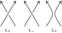
Figure 2. Knot polynomials
Note that the original diagram might be either L + or L -, depending on the chosen crossing's configuration. Then the Alexander–Conway polynomial, C(z), is recursively defined according to the rules:
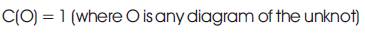

The second rule is what is often referred to as a skein relation. To check that these rules give an invariant of an oriented link, one should determine that the polynomial does not change under the three Reidemeister moves. Many important knot polynomials can be defined in this way.
The following is an example of a typical computation using a skein relation. It computes the Alexander–Conway polynomial of the trefoil knot. The shaded patches indicate where the relation is applied.
Figure 3 gives the unknot and the Hopf link. Applying the relation to the Hopf link where indicated,
Figure 4 gives a link deformable to one with 0 crossings (it is actually the unlink of two components) and an unknot. The unlink takes a bit of sneakiness.
Figure 5 implies that C (unlink of two components) = 0, since the first two polynomials are of the unknot and thus equal.
Putting all this together will show:
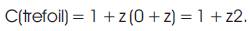
Since the Alexander–Conway polynomial is a knot invariant, this shows that the trefoil is not equivalent to the unknot. So the trefoil really is "knotted".
Actually, there are two trefoil knots, called the right and left- handed trefoils, which are mirror images of each other (take a diagram of the trefoil given above and change each crossing to the other way to get the mirror image). These are not equivalent to each other, meaning that they are not amphicheiral. This was shown by Max Dehn, before the invention of knot polynomials, using group theoretical methods (Dehn, 1914). But the Alexander–Conway polynomial of each kind of trefoil will be the same, as can be seen by going through the computation above with the mirror image. The Jones polynomial can in fact distinguish between the left and right-handed trefoil knots (Lickorish, 1997) (Figures 6 & 7).
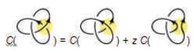
Figure 3. Hopf link
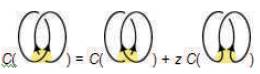
Figure 4. Unlink of two components
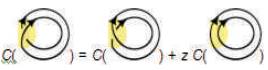
Figure 5. Unlink of two components
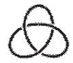
Figure 6. The left handed trefoil knot

Figure 7. The right handed trefoil knot
You can unknot any circle in four dimensions. There are two steps to this. First, "push" the circle into a 3-dimensional subspace. This is the hard, technical part which we will skip. Now imagine temperature to be a fourth dimension to the 3-dimensional space. Then you could make one section of a line cross through the other by simply warming it with your fingers. In general piecewise-linear n-spheres form knots only in n+2 space, although one can have smoothly knotted n-spheres in n+3 space.
In mathematics, a knot is defined as a closed, non-self-intersecting curve that is embedded in three dimensions and cannot be untangled to produce a simple loop (i.e., the unknot). While in common usage, knots can be tied in string and rope such that one or more strands are left open on either side of the knot, the mathematical theory of knots terms an object of this type a "braid" rather than a knot. To a mathematician, an object is a knot only if its free ends are attached in some way so that the resulting structure consists of a single looped strand.
A knot can be generalized to a link, which is simply a knotted collection of one or more closed strands. The study of knots and their properties is known as knot theory. Knot theory was given its first impetus when Lord Kelvin proposed a theory that atoms were vortex loops, with different chemical elements consisting of different knotted configurations (Thompson, 1867). P. G. Tait then cataloged possible knots by trial and error. Much progress has been made in the intervening years.
Schubert (1949) showed that every knot can be uniquely decomposed (up to the order in which the decomposition is performed) as a knot sum of a class of knots known as prime knots, which cannot themselves be further decomposed (Livingston, 1993). Knots that can be so decomposed are then known as composite knots. The total number (prime plus composite) of distinct knots (treating mirror images as equivalent) having , 1, ... crossings are 1, 0, 0, 1, 1, 2, 5, 8, 25, ... .
Klein proved that knots cannot exist in an even-dimensional space ≥ 4. It has since been shown that a knot cannot exist in any dimension ≥ 4. Two distinct knots cannot have the same knot complement (Gordon and Luecke, 1989), but two links can (Adams, 1994).
Knots are most commonly cataloged based on the minimum number of crossings present (the so-called link crossing number). Thistlethwaite has used Dowker notation to enumerate the number of prime knots of up to 13 crossings, and alternating knots of up to 14 crossings. In this compilation, mirror images are counted as a single knot type. Hoste, Thistlethwaite & Weeks (1998) subsequently tabulated all prime knots up to 16 crossings. Hoste and Weeks subsequently began compiling a list of 17-crossing prime knots (Hoste, Thistlethwaite & Weeks, 1998).
Finally the author listed some mathematical knots, they are as follows Unknot, Trefoil Knot, Figure-Eight Knot, Cinquefoil Knot, Three-Twist Knot, Stevedore Knot, 62 Knot, 63 Knot, Septafoil Knot, Endless Knot, Carrick Mat Knot, Perko Pair Knot, Pretzel Knot, Square Knot, Granny Knot, Prime Knot, Mirror Images Knot, Zero Knot, etc.
It is an ultimate purpose of knot theory to clarify a topological difference of knot phenomena in Mathematics and in Science. Based on the concept of mathematical knot theory and knot polynomial the researchers can give lot of suggestions in mathematics education. Knot theory is now one of the most active areas of Mathematics and it is the search for new applications.