Constant breadth curves were introduced by L. Euler in 1778 [12]. He studied the constant breadth curves in the plane. Then, many geometers have shown increased interest in the properties of plane convex curves. A brief review of the most important publications on this subject has been published by Struik [4]. Also, a number of interesting properties of plane curves of constant breadth are included in the works of Ball [16], Barbier [5], Blaschke [18] and Mellish [2]. A space curve of constant breadth was obtained by Fujiwara by taking a closed curve whose normal plane at a point P has only one more point Q in common with the curve, and for which the distance d(P;Q) is constant [13]. For such curves, PQ is also normal at Q. He also studied constant breadth surfaces. Furthermore, Köse presented some concept for space curves of constant breadth in Euclidean 3-space in [17] and M. Sezer investigated differential equations characterizing space curves of constant breadth and gave a criterion for these curves in [15]. Constant breadth curves in Euclidean 4-space was given by Mağden and Köse [1]. Corresponding characterizations for space like curves of constant breadth in Minkowski 4-space were given by Kazaz, Önder and Kocayiğit [14].

Furthermore, Reuleaux studied the curves of constant breadth and gave the method related to these curves for the kinematics of machinery [6]. Then, constant breadth curves had an importance for engineering sciences, particularly, in cam designs [10].

Bishop frame, which is also called alternative or parallel frame of the curves, was introduced by L.R. Bishop in 1975 by means of parallel vector fields. Bishop frame or parallel transport frame is an alternative approach to defining a moving frame that is well defined even when the curve has vanishing second derivative [3].

In this paper the authors give some characterizations of curves of constant breadth according to Bishop frame.

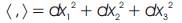
The Euclidean 3-space E³ provided with the standard flat metric given by

 

Where (x₁,x₂,x₃) is a rectangular coordinate system of 3 E . Recall that, the norm of an arbitrary vector a ∈ E³ is given by ||a|| =   γ is called a unit speed curve if velocity vector ν of γ satisfies ||a|| = 1.

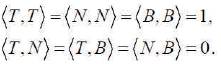
Denote by {T,N,B} the moving Frenet–Serret frame along the curve γ in the space E³ . For an arbitrary curve γ with first and second curvature, κ and τ in the space E³ , the following Frenet–Serret formulae is given as,

 

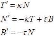
Where

 

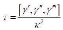
Here, curvature functions are defined by  Torsion of the curve γ is given by the aid of the mixed product

 

In the rest of the paper, the authors suppose every where κ ≠ 0 τ ≠ 0.

The Bishop frame or parallel transport frame is an alternative approach to defining a moving frame that is well defined even when the curve has vanishing second derivative. One can express parallel transport of an orthonormal frame along a curve simply by parallel transporting each component of the frame. The tangent vector and any convenient arbitrary basis for the remainder of the frame are used. The Bishop frame is expressed as

(1)

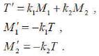
Here, they shall call the set {T, M₁ ,M₂} as Bishop trihedra k₁ and k₂ as Bishop curvatures.

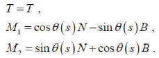
The relation matrix may be expressed as

 

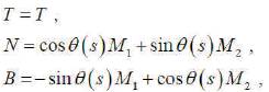
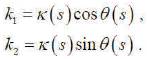
where θ(s) = arctan k₂ /k₁ ,τ(s) = θ'(s) and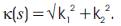

 

On the other hand

 

Suppose that k₁ , k₂ ,......k_n-1 are curvature functions of a curve α . A function H₁ : I → R defined by

 

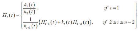
is called the i-th harmonic curvature function of α [8].

The characterizations of inclined curves in Eⁿ is given in [9] and [8] that

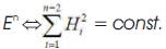• γ is an inclined curve in    and
• γ is an inclined curve in 

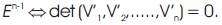
Let M⊂E³ is a curve given by (I,α ) chart. Then M is an inclined curve if and only if H(s) = k₁ (s)/k₂ (s) is constant for all s ∈ / [8]

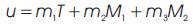
Let    be a simple closed curve in E³ space. These curves will be denoted by (C). The normal plane at every point P on the curve meets the curve at a single point Q other than P. They call the point Q the opposite point of P. They consider a curve in the class  as in [13] having parallel tangents T and T* in opposite points X and X* of the curve. A simple closed curve of constant breadth having parallel tangents in opposite directions can be represented by the equation

(2)

where X and X* are opposite points and T, M₁ ,M₂ denote the Bishop frame in E³ space [7].

We have from the equation (2)

(3)

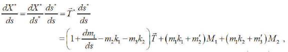
where k₁ and k₂ are the first and the second curvatures of the curve, respectively [7]. Since  they obtain

(4)

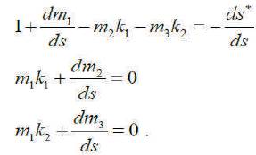
If they call Φ as the angle between the tangent of the curve (C) at point X(s) with a give fixed direction and consider dΦ /ds = k₁ , they can rewrite equation (4) as

(5)

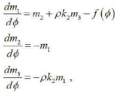
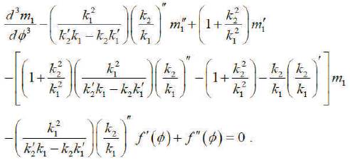
where f(Ф ) = ρ + ρ*, ρ = 1/k and ρ* = 1/k₁* denote the radius of curvatures at X and X*, respectively. And using system (5), 1 1 they have the following differential equation with respect to m₁ as

(6)

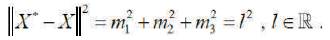
This equation is a characterization for X*. If the distance between the opposite points of (C) and (C*) is constant, then

 

Hence, they write

(7)

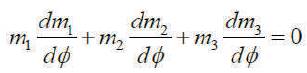
By considering system (5), they obtain

(8)

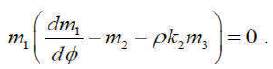
Thus the authors write m₁ = 0 or dm₁ /dΦ = m₂ + ρk₂ m₃ . Thus, we shall study in the following subcases.

dm₁ /dΦ = m₂ + ρk₂ m₃ . Then f(Φ) = 0. In this case, ( C*) is translated by the constant vector

(9)

of ( C). Now let us to investigate solution of the equation (6), in some special cases.

Suppose that X is an inclined curve. If we rewrite (6), they have the following differential equation:

(10)

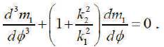
The general solution of this equation is

(11)

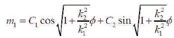
And therefore, they have m₂ and m₃ , respectively

(12)

(13)

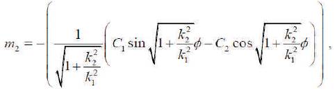
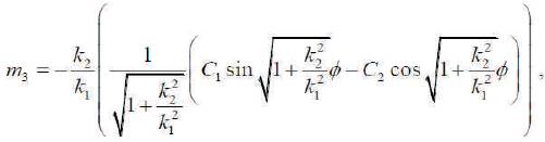
where C₁ and C₂ are real numbers.

Position vector of X* can be formed by the equations (11), (12) and (13). Also the curvature of X* is obtained as

 

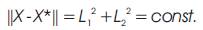
m₁ = 0. Then m₂ = const. and m₃ = const.. Therefore the position vector of X* can be written as follow:

(14)

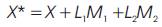
where L₁and L₂ are real numbers. Then the curvature of X* is obtained as

(15)

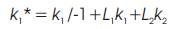
Hence distance between the opposite points of (C) and (C*) is

(16)