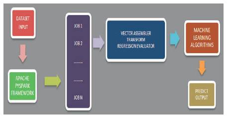
Figure 1. Framework Model for Prediction on Datasets using ML Techniques
Internet of Things (IoT), Big Data (BD), Artificial Intelligence (AI) and Machine Learning (ML) are the novel approaches where communication happens between man-made machines. Machines interact and acquire knowledge by implementing learning algorithms. Data analytics, prediction and classification methods are machine learning approaches applied on Big data for processing various unstructured data patterns. MapReduce is a widely used programming framework to parallelize these machine learning algorithms. To accomplish best outcomes, the algorithms are fine tuned using parallel practice. This technique uses MapReduce model for processing datasets multiple times by tuning the parameters as per the requirement. But this existing MapReduce model endures with high disk rates resulting in low throughput and inefficient time complexity. To achieve the minimal time consumption for tuning the jobs, Apache Spark framework replaces the MapReduce model. This is examined in this paper by evaluating the prediction on "Demand and Supply of India" dataset. A comparative analytical study is proposed in this paper to predict the demand for forecasting by training the existing data using tree based machine learning techniques. The prediction outcomes computed are compared on tree structured ML methods with respect to time and space utilization.
Big Data is lucid, enabling organisations to gain insights from new sources of data that were ever mined in the past. Processing data which varies in volume, variety and veracity is beyond the capacity of typical database software to intern, pile, control and evaluate (Logistic Regression, 2018). The exceptional trend of big data has a drastic impact on society and has an evident relation with diverse technological experts and end users in general. Data is expanding from various sources tremendously at the rate of generation. For instance, an International Data Corporation (IDC) report predicts that, from 2005 to 2020, the global data volume will grow by a factor of 300, from 130 Exabytes to 40,000 Exabytes, representing a double growth every two years (Apache Hive, 2014). This data which is transformed as information is anticipating for the new world (Stuart and Harald, 2007).
Recently, the increasing needs to gather massive amounts of data and aptitude to analyze the data in today's scientific and business world is competitive. Compute, transform, compress, extract and pile are the prominent challenges which convey the drawbacks in the conventional architecture and techniques (Lakshmi, 2016). MapReduce is an efficient parallel programming model for data intensive applications for processing big data sets (Tamano et al., 2011). Owing to few shortcomings in MapReduce, a standard approach is analysed and evaluated on highly scalable data. MapReduce uses a Hadoop distributed file system for parallel processing.
MapReduce models such as high disk reads and writes, low throughput result in low performance while handling clusters. Meanwhile there is express development in technology emerged platforms like Kafka, Spark, Flume and many more. Because of the drawbacks in MapReduce, upcoming technologies replaced it (Chu et al., 2006). The recent popularity of these parallel programming models has invoked significant interest in implementing scalable versions of Machine Learning algorithms.
Machine Learning can be defined as a “Field of study that gives computers the ability to learn without being explicitly programmed”. It is said to be science of algorithms where the machines are trained from examples, datasets, patterns, trends and experience through which output is automated. These algorithms are mechanized in performing either classification, categorization or forecasting outcomes from knowledge (Brownlee, 2016; Asha et al., 2013).
Depending upon the depth of knowledge that is available for learning, machine learning models can be categorized into supervised, unsupervised and semisupervised learning algorithms. Data classification, complex pattern recognition, predictions/intelligent decisions and clustering are the features of machine learning techniques through which they learn to understand complex data sets to make critical decisions and tune the features for abstracting high performance (Romsaiyud and Premchaiswadi, 2013; Pavlo et al., 2009).
MapReduce uses machine learning techniques for a single predictor. It demonstrates parallel map and reduces running of the jobs carrying iterative algorithm (Schwarz, 1978; Trabelsi et al., 2006). While this model results in high disk rates and low throughput, this can be improved by implementing the analytical model. This model implements comparative analysis using Spark Framework replacing the existing MapReduce on machine learning algorithms.
To build a scalable machine learning model that provides performance on very huge datasets using spark framework for prediction analysis. Hand-tuned tree based machine learning techniques are comparable in their implementation measuring their efficiencies in terms of space and time.
Data analysis using machine learning systems examine the datasets and involuntarily capture the features while processing the trial data. The training data consists of input items and expected outcomes (Manar and Stephane, 2015). The result of the function can be an uninterrupted value, or it predicts a class label of the input object. The task of the learning machine is to forecast the value of the task for a valid input object having a small number of training data (Hadoop – MapReduce, 2018; Logistic regression, 2018).
The workflow of the proposed model in Figure 1 is drafted (Lakshmi, 2017) as below:
Figure 1. Framework Model for Prediction on Datasets using ML Techniques
Step 1: Read the data in spark data frame and use time method to invoke time.
Step 2: Splitting the data into train data and test data using random Split function from spark.
Step 3: Vector Assembler converts the data in terms of vectors.
Step 4: Transform function modifies the vectors into necessary data frames.
Step 5: Mapping the labelcol and featurecol using methods from MLlib.
Step 6: Pipeline consists of stages, each one operate as an estimator or a transformer when fit() is initiated.
Step 7: Regression Evaluator is used to evaluate the prediction on the featured data.
Step 8: Random Mean Square Error (RMSE) is calculated to find the mean square error.
Step 9: Total evaluated time complexity is evaluated to process the data set.
Forecasting from data, study of observations, learning patterns and constructing the algorithms can be explored using machine learning (Bowles, 2015; Caruana et al., 2008). These algorithms can be operated by developing a framework for trained input data set to make data driven predictions and decisions rather than following a static way of programming implementation dynamically.
Machine learning models incorporate statistical techniques for handling regression and classification tasks with multiple dependent and independent variables. There are variuos regression techniques available for predicting outcomes (Bowles, 2012).
Spark uses function pipeline to interpret the learning flow for implementing machine learning techniques. This learning flow is implemented on datasets to process the training data for attaining best test results.
Tree based machine learning techniques such as Decision Tree, Random Forest and Gradient Boosting tree are used for prediction analytics. Data set considered for analytics is taken as Domestic supply of Indian economy with respect to food items cereals, wheat, maize, barley, rice, vegetable-oil, meat, poultry, fish-sea food, egg, milk, vegetables, sugar-crop and fruits since 1940. The data set consists of the quantity used for the past 70 years. This model tunes the dataset for analysing the prediction for further years through which domestic supply can be forecasted.
Decision tree is one of the most widely used and practical methods for inductive reference. It is a method for approximating discrete valued functions that is robust to noisy data and capable of learning disjunctive expressions (Romsaiyud and Premchaiswadi, 2013). Each rule is represented as if-then rules to improve readability. These learning methods are among the inductive inference algorithms applied learning to analyse and diagnose different cases for best output prediction or classification.
This algorithm is developed from core algorithms and this is exemplified by the Iterative Dichotomiser 3 (ID3) algorithm. The central choice in the ID3 algorithm is selecting which attribute to test at each node in the tree. As a good quantitative measure, an attribute is defined upon statistical property called information gain. The defined measure for calculating the information gain is entropy that characterizes the purity of an arbitrary collection. The tree concentrates on interpretability by suggesting a breakdown for making a decision.
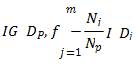
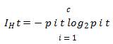
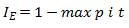
where, IG is Gini Index, IH is entropy and IE is the classification error defined for all non empty classes.
F is the feature to perform split. DP and Dj are the datasets of the parent and jth child node, I is out-impurity measure. Np – Total number of samples at the parent node and Nj is the number of samples in the jth child node. IG computes the difference between the impurity of the parent node and the sum of the child node impurities. Maximum IG can be obtained if the impurity is low in the child nodes. Binary decision tree can be thoroughly examined using 3 measures viz., Gini Index (IG ), Entropy (IH ) and Classification Error (IE). The entropy criteria attempt to maximize the mutual information in the trees observing the proportion of the samples of a particular node t.
Gini Index is said to be a criterion used in order to minimize probability of mis-classification.
Using the decision tree, the process begins at the root and follows by splitting the data by information gain. It is an iterative process for reaching the maximum depth of the tree. The tree is pruned in the process by implementation. Decision tree feature selection and prediction from the training data is exemplified in Figure 2.
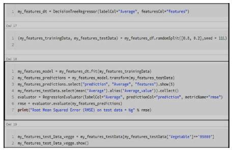
Figure 2. Decision Tree in Jupyter Notebook
Figure 3 describes the output prediction values for the corresponding average supply for the fruits feature.
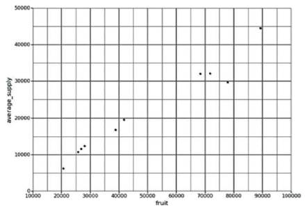
Figure 3. Graph Representing Average Supply for Fruits Feature
Random forest is an ensemble learning method which constructs numerous decision trees. It builds a robust model that has a better generalization error, and is less susceptible to overfitting. These trees use both classification and regression methods for forecasting the future output for given feature selection.
Random forests are amalgamation of various decision tree predictors where each tree depends on the values of a random vector. This vector is autonomously modelled with the unique feature distribution involving all trees in the forest. The use of law of large numbers makes the model efficient by avoiding over fitting. The randomness property builds precise classifiers and regressors.
Each tree is grown as follows:
Bias variance tradeoffs are controlled by opting large value of n and by decreasing the randomness which is likely to over fit. In this implementation, Random Forest Classifier, the model range of the bootstrap sample is chosen to be equal to the figure of samples from the original training set by executing d = √m, where m is the quantity of features in training set.
Figure 4 constructs the random forest classifier from each decision trees via then_estimator parameter and used the entropy criterion as an impurity measure to split the nodes.
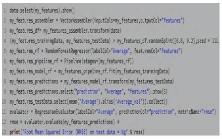
Figure 4. Random Forest in Jupyter Notebook
Gradient Boosting classifier or regressor receives predictive output by implementing boosting technique for non linear regression as shown in Figure 5. This improves the precision by concerning weak classification algorithms for incrementally transformed data. To ensemble weak predictions, series of decision trees are created in order to improve accuracy (Lakshmi, 2016; 2017).
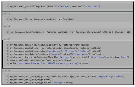
Figure 5. Gradient Boosting Tree in Jupyter Notebook
The gradient boosting method generalizes tree boosting to minimize the loss function for the regression. For further improvement, the model incorporates randomization to prove the approximation precision and execution pace of gradient boosting. Regression with loss function L is given as a general procedure by differentiating the loss function with an initial model F(x).
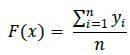
This initial model iterates until the model converges by calculating negative gradients – g(x ) to fit tree h.
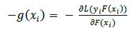
The iterative function is given in equation (6), where ρ= 1 and h is a tree:

Specifically, this algorithm iterates at each draw on a subsample of the training data randomly (without replacement) from the full training data set.
The square loss function for regression problem which is robust to outliers is given in equation (7).
The model is revised for the existing iteration by arbitrarily choosing a sub sample by replacing the actual sample to fit the base learner. Gradient Boosting Tree approach increases robustness besides congestion of training sets.
Tree based machine learning algorithms are used for processing large temperature data set. The efficiency is observed by comparing MapReduce with Spark framework. The performance is evaluated on time and space as factors for interpreting the results.
The MapReduce model shows high disk rates for read operation at 17.23 MB/sec and writes operations at 19.41 MB/sec. This even reduces the performance of a processor. But while executing the jobs on Spark platform, the results are 28.65 MB/sec on read and 38.43 MB/sec for write operations. From Table 1, it is clear that the Time and Space utilized by MapReduce is additional when compared with Spark.
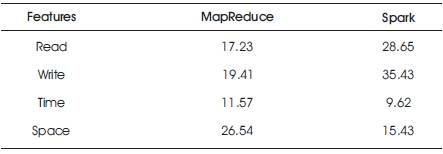
Table 1. Metrics of MapReduce and Spark
The machine learning techniques reveal the efficient use of time and space. These methods train machines, so that they adapt to the dataset. Figure 6 shows the combined measures of learning techniques considering the time, space, read and write operations.
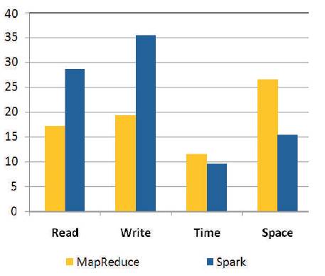
Figure 6. MapReduce and Spark Performance
Table 2 gives the tree based machine learning techniques used in performance evaluation. To evaluate the best prediction outcome, tree based machine learning algorithms are considered. Each algorithm predicts the outcome. The output is analysed by their performance with respect to time, space, read and write operations. Table 2 gives the basic analysis throughput which is more from random forest. Time and space complexity is best shown from Gradient Boosting tree and Decision tree respectively.
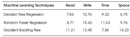
Table 2. Measures using ML Techniques
Machine learning methods are compared with respect to Time, Space, Read and Write operations using Gradient Boosting Tree, Decision Tree and Random Forest techniques which is shown in Figure 7.
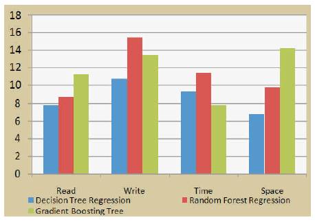
Figure 7. Machine Learning Methods
The prediction taken from the techniques is given in Table 3. This gives the deviation in measures of machine learning methods to that of average supply required for various years. The observed analysis depicts that Gradient Boosting tree utilizes additional space when compared with Random forest and Decision Tree. Time is another feature where Random forest and Decision tree complexity is short.
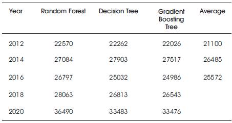
Table 3. Prediction Measures against Average
From Table 3, it is evident that Random Forest gives the nearest predictions with reference to the average computed from previous years. The Random Mean Square Error (RMSE) taken is drafted in Table 4 for the tree based algorithms.
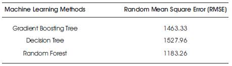
Table 4. RMSE for ML Techniques
The prediction calculated by the model is enacted in Figure 8, whereas RMSE (Random Mean Square Error) is computed for the deviations taken from average to that of the prediction calculated as shown in Table 4, and is represented in Figure 9.
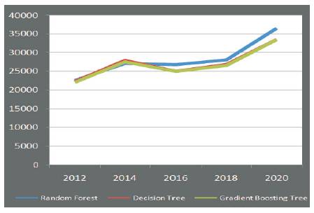
Figure 8. Predictions Drawn from Machine Learning Methods
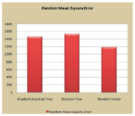
Figure 9. RMSE Computed from the Machine Learning Algorithms
The observation illustrates the performance of the tree based learning algorithms. RMSE, one of the measures for analytical evaluation reveals Random Forest has minimal error when compared with the other tree based learning algorithms. So, the predictions drawn from random forest are more accurate.
Executing Data analysis, jobs using various parameters are observed in machine learning for efficient time and space. The proposed model optimizes the machine learning techniques on a distributed environment using spark framework to minimize the total execution time and space for future predictions. The proposed model uses Apache Spark and Python as Application interface by distributing the jobs in evaluating time and space complexities for prediction.
This model for prediction can merely motivate in incorporating some more additional features such as humidity, moisture, fog and pollution consistency to identify better estimate of temperature for future analysis. Much of these models are used due to the exponential growth in computing power, which allows gradually for choosing the best resulted model.