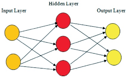
Figure 1. A Simple Neural Network
Image recognition has many applications today, and is being done by using various methods and technologies. Neural networks are now popularly used for various image processing applications. QCNN (Quaternion Convolutional Neural Networks) and CNN (Convolutional Neural Networks) are two methods that can be used for image recognition. In this paper, we compare performance of QCNN and CNN in colour image recognition. It shows that QCNN can easily capture the inter pixel relations producing better RGB images whereas CNN produces worst gray scale images.
Image recognition, a popular application of image processing is a process of identification of different objects, colours, humans, animals, numbers, texts, etc. having wide applications in heterogeneous images as they contain different objects, colours and texts.
A model in image recognition is considered good, if it is able to extract global and hidden relations between pixels as well as RGB components of a single pixel. Also, a good model should efficiently encode relations within the input features and should detect the shape, width, size and colours of different objects in the image.
Among researchers in this field, neural networks has gained a better position due to various applications in image recognition methods. CNNs are better performers in image processing as these models have been successful in solving various simple and complex pattern of images.
In this paper we propose another type of neural network which includes quaternion,called as QCNN. Quaternions are the hyper-complex numbers that includes one real part and three imaginary part which can be matched in three and four dimensional feature vectors perfectly. We claim that these quaternions can better visualize the global and local dependencies of the pixels than CNNs and can recognize the objects in a more efficient way. QCNN requires only one fourth parameters used by CNN, which is another advantage of QCNN over CNN.
The main objectives behind this experiment is to show how QCNN is able to recognize RGB component of the colour image as well as to show the impact of Hamilton product in the image recognition which is the main characteristic of QCNN (Dataman, 2018).
In this experiment we take various heterogeneous colour images. We give the input image to both QCNN and CNN models, find the output, then decide the region of interest of the output image, zoom it and give the final resultant output. Our objective in this experiment is to show that an object colour and text colour is perfectly recognizable by QCNN whereas CNN is not able to recognize the colour and produces black and white images.
We also compare and analyze the difference between the results of QCNN and CNN by PSNR (Peak Signal to Noise Ratio) and SSIM (Structural Similarity). From this we will show that QCNN produces better PSNR and SSIM (in percentage) based image as that of CNN.
According to He et al. (2016), neural network models are the heart of the different image recognition methods. It can recognize both basic and complex patterns in image. In most of this case deep convolutional neural networks are used.
According to Sangwine (1996), QCNN is an appropriate method to develop multi-dimensional input features. Fourier transforms are a fundamental implementation in signal and image processing. But, until recently, there was no explanation of a Fourier transform applicable to colour images in a holistic manner. Hyper-complex numbers, especially quaternions, can be adapted to define a Fourier transform applicable to colour images. The properties of the transform are developed, and it can be shown that the transform may be computed utilizing two standard intricate fast Fourier transforms. The resulting spectrum is interpreted in terms of familiar phase and modulus concepts, and an incipient concept of hyper-complex axis.
Adam optimizer is used in this model according to the suggestion of Kingma and Ba (2015). They used stochastic gradient-based optimization, which has basic practical importance in many fields of engineering. The hardtanh activation function is used according to Collobert (2004).
Simple Neural Networks are the networks consisting of multiple neurons. It may be organic or artificial in nature. In neural networks, there is no requirement of reorganization of output as it can easily modify the changing input. A simple neural network has input layer, hidden layer and output layer as shown in Figure 1.

Figure 1. A Simple Neural Network
Neural networks acts as human brain. The neurons are like a mathematical function that represents different features and it works as the architecture of the model. Input layer contains input features. Hidden layer takes the input weights and compares the results with the expected output. It will modify the input weights until the error is minimum.
CNNs are the type of neural network which performs convolution operation between input image and kernels or filters (Ganesh, 2019). CNN consists of four layers as explained in Figure 2.
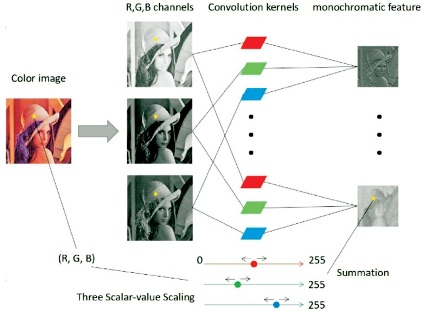
Figure 2. Illustration of CNN On Convolution Layer (Zhu et al., 2018)
This is the first layer of CNN which is a very important layer as it extracts the feature map of the input layer. It draws out the input characteristics by convolution operation between input layer and kernels. Since here we do operations in image and pixels, we can call it as a discrete convolution or simply we can call it as the dot product between the input and kernels in case of vector. If there are two functions named C1(x) and C2(x), then the convolution between two functions is mathematically represented as in Equation (1).

This is the second layer of CNN in which we apply different activation and cost functions. Different types of activation functions are ReLu, sigmoid, hardtanh, softmax, tanh, softsign, etc. (Socher & Mundra, 2015). In case of CNN, in this experiment, we use hardtanh activation function. The objective of using activation function is to activate a neuron that will fire to the next neuron when a particular value is applied. We can use different activation functions as per our requirement and convenience (Arena et al., 1994).
To shorten the training time and reduce the number of parameters we use pooling layer which reduces the size of input as well as conserve the required information. It is like convolutional layer where more filters are applied to recognize different relevant informations.
It is the last layer where the output of the pooling layer is converted into a one dimensional vector. In this experiment we use tmax activation function. This function is generally preferred in case of image classification or image recognition which gives the probabilities of an object present in an image belong to a particular class.
QCNN is a type of neural networks which is operated using quaternions. Quaternion means a value is divided into four parts containing one real part and three imaginary parts which acts as vectors. So it is a hyper complex number which means an extension of a complex number in four dimensional space. A quaternion q is therefore defined as in Equation (2).

Where r, a, b, c are the real numbers and 1,i,j,k are the Quaternion Unit basis. r is taken as real part whereas a, b, c, are the imaginary parts with i2 =j2 =k2 =ijk=-1.
Quaternion Conjugate of q is given by:

Quaternion Norm of q is given by:

Normalized Quaternion of q is given by:

Like CNN, QCNN has also four layers. Before convolutional layer, the number of input features are taken in the form of quaternion which has four components. So, the input features in Quaternion space become one-fourth of the input features in real space.
It is the first layer of QCNN, instead of using convolution operation, we use Hamilton product between the input and kernels. We use dot product in case of CNN and Hamilton product in case of QCNN.
If there are two quaternions q1 and q2, then they can be represented as:
q1 = r11+a1i +b1j+ c1k
and

The Hamilton product between these two quaternions is given by:
q1x q2 = (r11 + a1i +b1j +c1k) x (r21 + a2i+b2j+c2k)
= (r1r21 + r1a2i + r1b2j + r1c2k) +(a1r2i – a1a21+a1b2ka1c2–j)+
b1r2j–b1a2k–b1b21+b1c2i)(c1r2k+c1a2j–c1b2i–c1c21)
By arranging the above expression we get,

The kernels are represented in terms of different weights. These weights extract different latent relations by performing Hamilton operation with the input layers as shown in Figure 3. So in QCNN, the input is represented as:
qin = rin1 + aini + binj + cink
k and weights in quaternion form is given by:
w=wr+wa+wb+wc
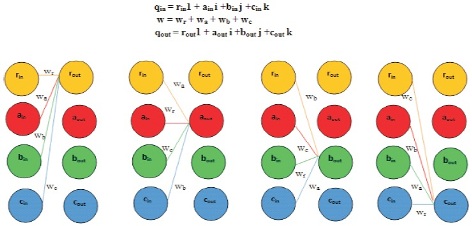
Figure 3. Hamilton Product between Input Layer and Weight (Parcollet et al., 2019)
So the Hamilton product between qin and w gives the output value in quaternion as qout .

In general, if (x,y) is the co-ordinate of the new feature map and w is the new quaternion weight, then this can be written as:

where, S’xy = Pre-activation quaternion output at layer l and γ = Quaternion input at previous layer.
Likewise CNN, in this layer different activation and cost functions are applied to the pre-activation output of QCNN. For QCNN, we also apply hardtanh activation function. For applying activation function, split are arranged in the form of one dimensional vector.

where,α=Quaternion split activation
The back propagation algorithm applied by the method is generally used in neural networks by gradient descent method. It calculates the gradient of the error function with respect to weights (Nitta, 1995).
It is somehow similar to the pooling operation in CNN where max pooling, average pooling (mostly preferred) are applied. It helps to preserve more relevant data present in the input.
It is the last layer where the results after the pooling layer is mathematically expressed as one dimensional vectors.
Before the final output the number of features in quaternion space is converted into real space and therefore the number of output features becomes four times. Figure 4 explains the layers of QCN.
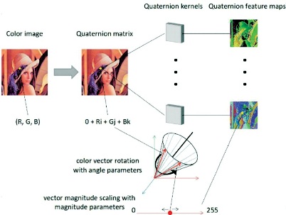
Figure 4. Illustration of QCNN On Convolution Layer (Zhu et al., 2018)
QCNN and CNN have almost same layers and topology. The first difference is that in QCNN instead of applying convolution we use Hamilton product and other difference is we take the input in the form of quaternion. If we focus the second difference we can understand that if the number of input characteristics is, for example 32, then in quaternion it becomes one fourth, i.e., 8. So, the number of inputs given to QCNN is less than that of CNN. In QCNN, we convert a value from real space (R-space) to quaternion space (H-space) (Madali, 2020).
After all the operations in all layers of QCNN as discussed, in last layer we convert the output in H-space to R-space. In other words, for 8 output features, the number of output characteristics becomes 4 times i.e.,32.
Here, we introduce the encoder-decoder model of QCNN as QCAE and for CNN as CAE. Here, the convolutional and transposed convolutional layer of QCAE and CAE acts as encoder and decoder respectively.
In case of QCAE, there are almost 6400 parameters where as for CAE it is 25000. Talking about dense layers, for QCAE, the numbers of input and hidden layers are 256 and 256 respectively whereas for CAE, it is 1024 and 1024 respectively. So for QCAE, number of dense layers becomes 256 x 256 nearly equal to 0.26 M whereas for CAE, it is1024 x 1024 nearly equal to1M.
In this experiment, both models are trained to produce gray scale image similar to the gray scale training image and then fed to the validation colour images to reproduce final output. In this experiment we used one training image and two validation datasets. Training image is converted to gray scale image whereas validation image is converted to gray scale image. Training and validation images can be taken randomly. The training and validation images taken in this experiment are shown in Figure 5.
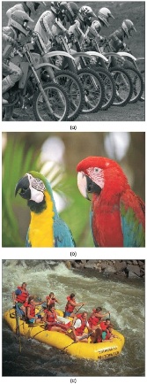
Figure 5. Training and Validation Image Taken (a) The Training Image (Gray Scale Image) (b) Parrot Image (RGB Image as Validation Image-1) (c) Sailor Image (RGB Image as Validation Image-2)
Training of models is performed by taking 768 x 512 dimensional gray scale images. We also take two 768 x 512 dimensional colour validation datasets. The value of gray scale pixel is taken in the form of quaternion by concatenating this value three times. Same process is repeated for CAE also. The quaternion value extracted in this process can be written mathematically as:

where, Ix,y =Pixel value of image I at (x,y)
GS =Gray Scale value.
The RGB value obtained during the processing of validation image is also repeated three times for both QCAE and CAE. Mathematically, it can be represented as,

where R represents Red, G represents Green and B represents Blue. While taking the data both in case of training and validation datasets, the real value of quaternion is taken as 0.
Training is done during 3000 epochs with Adam optimizer (Kingma & Ba, 2015), vanilla hyper-parameters. The learning rate in this experiment is taken as 5-4. The hardtanh activation function is used in both QCAE and CAE in both convolutional and de-convolutional layers. Quaternion parameters are initialized according to the value explained in Parcollet et al. (2018). Finally the input image is given to both QCNN and CNN and output of both models are obtained. Then objects are cropped from output image and are focused. Both the results are compared visually as well as by using comparison parameters PSNR and SSIM.
Comparison is very much important in research. Comparison tells us about the efficiency, goodness of one process compared to other processes. Without comparison parameters we will not able to know which is better. So at different times we use different parameters to compare two or multiple processes and reach to a conclusion. In this experiment we use PSNR and SSIM to reach the conclusion of which is better between QCNN and CNN.
It compares the input image and resultant image (generally compressed or reconstructed images) by calculating the ratio of signal to noise. It is measured in decibel (dB). It generally shows the quality of resultant image. Higher the value of PSNR is considered as the good indication of the output image. Mathematically:

where, F= Maximum Fluctuation in input image
MSE= Mean Squared Error

where, I1(x,y) = Intensity at pixel location (x,y) of image-1
I2(x,y)=Intensity at pixel location (x,y) of image-2
It gives the idea of how much percentage of data is recovered at output.
Figures 6, 7, 8, 9, 10, and 11 show the results for images 1, 2, 3, 4, 5, and 6 respectively. These Figures compare the CAE and QCAE produced image.
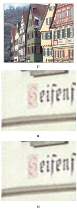
Figure 6. Results of Image-1 (a) Input Image (b) CAE Produced Image (c) QCAE Produced Image
In Figure 6 for Image-1 we can see that the writings on the house is written in both red and black colour which is correctly detected by QCAE but CAE produced image cannot detect the colour of the writings.
In Figure 7 for Image-2, flower colour is clearly revealed as red in case of QCAE but CAE cannot distinguish the red flower colour and produces gray scale image.
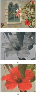
Figure 7. Results of Image-2 (a) Input Image (b) CAE Produced Image (c) QCAE Produced Image
In Figure 8 for Image-3,the yellow colour of the hat is produced in QCAE but CAE cannot catch the yellow colour.
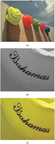
Figure 8. Results of Image-3 (a) Input Image (b) CAE Produced Image (c) QCAE Produced Image
In Figure 9 for Image-4, the number 32 is exposed correctly by both QCAE and CAE but the door colour is noticed by QCAE as brown but CAE produces its colour as silver.

Figure 9. Results of Image-4 (a) Input Image (b) CAE Produced Image (c) QCAE Produced Image
In Figure 10 for Image-5, yellow and blue colour is spotted by QCAE where CAE fails to capture this colour.
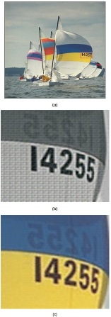
Figure 10. Results of Image-5 (a) Input Image (b) CAE Produced Image (c) QCAE Produced Image
In Figure 11 for Image-6, 20042 text is written in green which is caught correctly by QCAE while CAE cannot identify it.

Figure 11. Results of Image-6 (a) Input Image (b) CAE Produced Image (c) QCAE Produced Image
Tables 1 and 2 compare the PSNR and SSIM parameters for different images of both QCAE and CAE. Table 1 concludes that PSNR value of CAE produced image is more than CAE produced image. But Table 2 shows that SSIM of QCAE is much better than CAE.
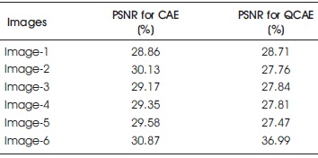
Table 1. PSNR Comparisons of QCAE and CAE
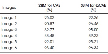
Table 2. SSIM Comparisons of QCAE and CAE
In this paper, an unique method of quaternion called as quaternion convolutional encoder-decoder has been presented. Also the image recognition operation in real convolutional network has been performed. From these different results, we can easily conclude that QCAE produces better results as compared to CAE. The credit of this good result goes to Hamilton product. This experiment also demonstrates that the QCAE can perfectly catch the inter pixel internal, local and global relations between the input features whereas CAE completely fails to identify it. So, QCAE is better in terms of detecting colours as well as texts. Our future work will include the quality compression of various heterogeneous images.