(1)
Synthetic Aperture Radar (SAR) imaging has been an exciting field owing to its wide application in military/non military fields. This paper is aimed at investigating effects of using different types of signals and emission parameters on the accuracy and resolution of simulated SAR image and performing simulation on a reconstructed SAR image of an fully polarimetric SAR for identifying different land features. The speckles in the image are removed using the Lee filter and then the image is decomposed using Pauli decomposition method. After feature extraction, neural network techniques are used for training, validating and testing the network. The final image classified in RGB, representing features like urban, vegetation and water has been achieved. The percentage classification of each feature pixels in the image has been presented using confusion matrix.
Synthetic Aperture Radar (SAR) are coherent radars which are mostly airborne or space borne systems that uses the flight path of the platform to simulate an extremely large antenna or aperture electronically thereby generating high resolution images (Berens, 2006; Chan & Koo, 2008). An established SAR simulation system using MATLAB can be helpful in understanding the SAR principles and optimal design of SAR system before hardware realization. The choice of parameters can be tested for optimal designing. SAR have wide range of application in military as well as commercial purposes like airborne reconnaissance, surveillance etc., (Wei, 2009). Various types of SAR include Stripmap, Spotlight, Interferometric and Inverse SAR. Imaging radars generate surface images that are very similar to images produced by instruments that operate in the visible or infrared parts of the electromagnetic spectrum. Visible and infrared sensors use a lens or mirror system to project the radiation from the scene on a “twodimensional array of detectors”, which could be an electronic array or, a film using chemical process. The look of both images is different as they are collected using entirely different principles. The pixels closer to eye have finer resolution in case of optical imaging whereas pixels farther from SAR have finer resolution (Skolnik, 2008; Curlander & McDonough, 1991). The main factor for the evolution of SAR is the thrust for better resolution. In case of Real Aperture Radars (RAR), the larger the antenna, the finer the resolution achieved as the track resolution is determined by the beam width while the cross resolution is determined by pulse width. In SAR, using the antenna phase array theory, an antenna aperture can be created or represented from multiple point sources. SAR exploits this physics by taking a single moving antenna and using it to take a line of images mimicking multiple point sources (Kent et al., 2007).
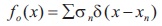
An ideal target function, which represents range-domain function range, and reflectively of the targets in the x (range) domain is given by Soumekh (1999).
δ is the Dirac delta function.
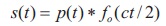
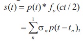
The received echoed signal is,
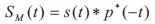
The optical reconstruction method is based on matched filtering. The time domain convolution, denoted by the first asterisk in Equation (3), is the operation that produces SM(t), where p*(-t) is the matched filter impulse response, and the second asterisk denotes complex conjugate.
The simulation model for execution of simulations is as per Figure 2, for all the three types of signals.
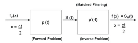
Figure 1. System Model for Range Imaging
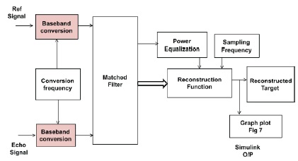
Figure 2. Block Diagram for Range Imaging Simulation
The simulation is based on a simple rectangular sinusoidal pulse of duration Tp given by,
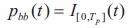
where I [0,Tp] (t) is the indicator function. This produces a baseband pulse pbb of duration Tp. This baseband pulse is p then up converted and expressed as an analytic signal as,
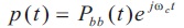
ωc is the carrier frequency in radians/second. The signal in c Equation (5) is then emitted from the transmitter antenna and reflected off the targets represented by Equation (6), resulting in a received signal echo.
The reflected signal is then returned to its baseband form,
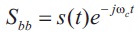
The magnitude of Sbb is plotted against the range domain sample spacing which produces Figure 4, the baseband echoed signal. A matched filter is then used in conjunction with the baseband echoed signal to produce, SM(t), the range reconstructed target function via matched filtering as shown in Figure 6.

Figure 3. Baseband Referance Signal
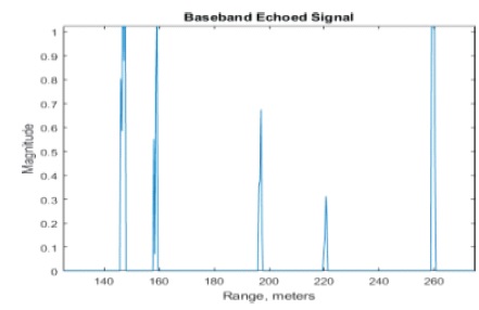
Figure 4. Baseband Echoed Signal
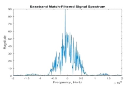
Figure 5. Matched Filtering Signal Spectrum
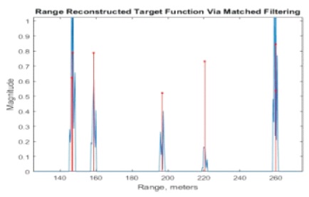
Figure 6. Reconstructed Image
The second type of signal, Linear Frequency Modulated (LFM) signal is generated similar to the sinusoidal pulse. The LFM chirp signal in this simulation is linearly increasing in frequency and thus called an “up-chirp” whose analytic signal is given by:

where ωcm is the modified carrier frequency and ωc is the unmodified carrier frequency in radians per second, and a is the chirp rate in radians per square (Fason, 2013).
The carrier frequency, pulse length and target scene composition were kept constant for all three types of signal for simulations. The bandwidths and energies of all the three signals used are similar, but not equal. All three signals have correctly found the ranges of the targets. The linear frequency modulated chirp signal had the finest range resolution for the selected simulation parameters; same is evident by the minimal width of the main lobes in Figure 7. The noise pulses were although able to accurately identify the range but found lacking in reflectivity parameter of the targets.
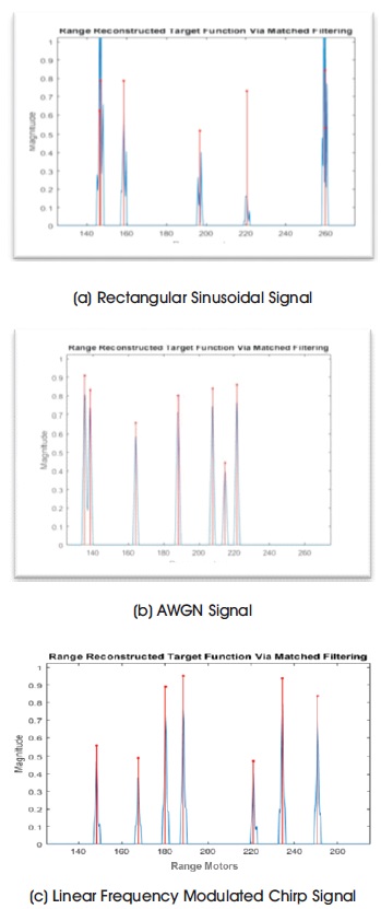
Figure 7. Image Analysis with Different Techniques
Let us define an ideal target function in the same manner as done for range imaging, i.e., with lumped targets represented using the Dirac delta function.
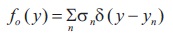
where σn is the nth target reflectivity.
The echo signal is given by,

k = ω/c is called the wave number. Applying a baseband conversion to Equation (10), the final reflected signal is produced. Forward/reverse signal for cross range resolution imaging is given in Figure 8.
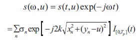
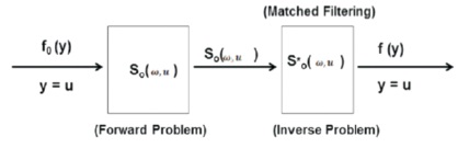
Figure 8. Forward / Inverse System Models for Cross Range Imaging
The coding for carrying out simulation uses the existing codes available in crange files available in MATLAB. The factors that determine the bandwidth and thus affect the resolution are the size of the synthetic aperture 2L, radar frequency and target range. The factors affect the crossrange resolution by artificially increasing the effective bandwidth of the transmitted signal through the slow-time Doppler filter. With larger effective bandwidth the signal space can get more number of samples.
The cross-range resolution has been simulated using three cases by varying the key parameters as shown in Figure 9.
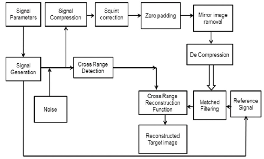
Figure 9. Block Diagram for Cross Range Imaging Simulation
Case I - Normal Resolution: The baseline for this simulation with respect to its resolution has been achieved with the help of parameters for the transmitted radar pulse and the system geometry.
Case II - Low Resolution: There is a reduction in resolution by moving the target area further away from the synthetic aperture, resulting in lesser number of samples than in the baseline case and subsequently a lower resolution.
Case III - High Resolution: Greater resolution is achieved than in case of baseline by increasing the carrier frequency, thereby increasing the number of samples taken.
The importance of physical parameters in case of crossrange imaging have been demonstrated in Figure 10, 11 and 12 for normal, low and high resolution respectively. The parameters which were tested and simulated were carrier frequency (fc), distance to target area center, size of the c synthetic aperture (2L). With the increase in the carrier frequency or size of the synthetic aperture and how far the aircraft mounting the transceiver moves while completing transmit/ receive cycles, the corresponding bandwidth in the slow-time Doppler filter increase resulting in finer resolution. Conversely, if we reduce the distance to the center of the target area, thereby effectively increasing the bandwidth of slow-time Doppler filter and in turn achieving better resolution. Also by increasing the carrier frequency, the signal energy required to achieve higher resolution is also increased.
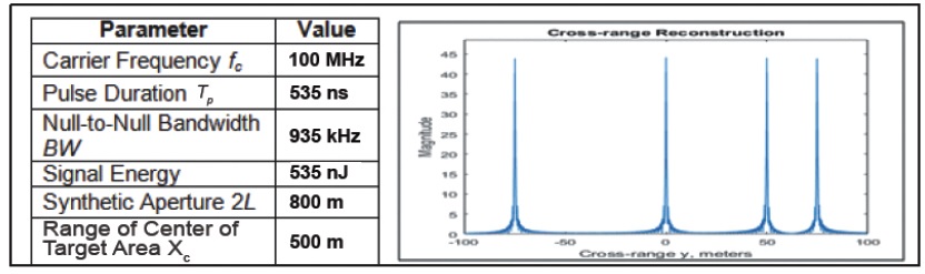
Figure 10. Image Reconstruction with Normal Resolution via Matched Filtering
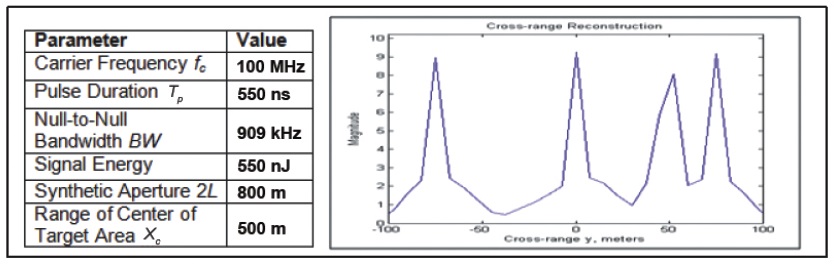
Figure 11. Image Reconstruction with Low Resolution via Matched Filtering
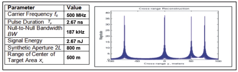
Figure 12. Image Reconstruction with High Resolution via Matched Filtering
The radar transmits a wave of one polarization and receives echoes in two orthogonal polarizations simultaneously. This is followed by transmitting a wave with a second polarization and again, receiving echoes with both polarizations simultaneously as shown in Figure 13. In this way, all four elements of the scattering matrix are measured.
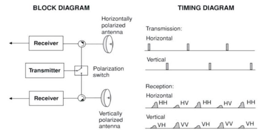
Figure 13. Block Diagram of PolSAR
The MATLAB simulation for classification of geographical feature is explained with the help of the block diagram as shown in Figure 14.
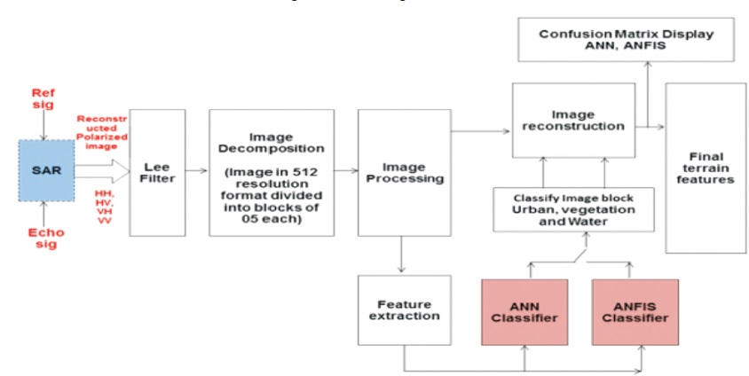
Figure 14. Design Flow Chart of Classification
Image classification of SAR using neural network are as follows :
ANN classifier is applied to the extracted image. ANN is to find the most appropriate grouping of training, learning and transfer function for classifying the data sets with growing number of features and classified sets. The different combinations of functions and its effect while using ANN as a classifier is studied and the correctness of these functions are analyzed. The image has been classified into three features i.e., Urban, Vegetation and Water. Now part of the image is used for training of the network and part will be used for testing and validation once network is trained. The block diagram depicting the ANN classifier with different types of layers (hidden layer 2, input and output layer) is shown in Figure 15. The weight and bias are used to achieve the condition when mean square error is minimum. Given separate sets of input and output data, genfis2 generates a FIS using fuzzy subtractive clustering. genfis2 accomplishes this by extracting a set of rules that models the data behavior. The rule extraction method first uses the SUBCLUST function to determine the number of rules and antecedent membership functions and then uses linear least squares estimation to determine each rule's consequent equations. The fuzzy_classifier (train_data, train_class, test_data) and fuzzy_process (X, c, options, init_V) are used for Adaptive Neuro Fuzzy Interface System (ANFIS). The same result will be validated by the confusion matrix. The confusion matrix for both ANN and ANFIS are generated. The confusion matrix tells us the percentage distribution of target class in the output class. The result of the confusion matrix will be analyzed separately.
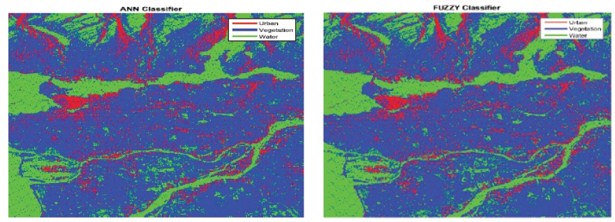
Figure 15. Images Classification by ANN/ Fuzzy Classifier
The confusion matrix for ANN and ANFIS classifier are shown in Figure 16. The rows of the confusion matrix correspond to the output class or the predicted class and the columns correspond to the target class or true class. The diagonal cells communicate to pixels that are correctly classified. The off diagonal cells correspond to inaccurately classified pixels. The area under observation has following percentage coverage for each class after 07 epoch as shown in Table 1.
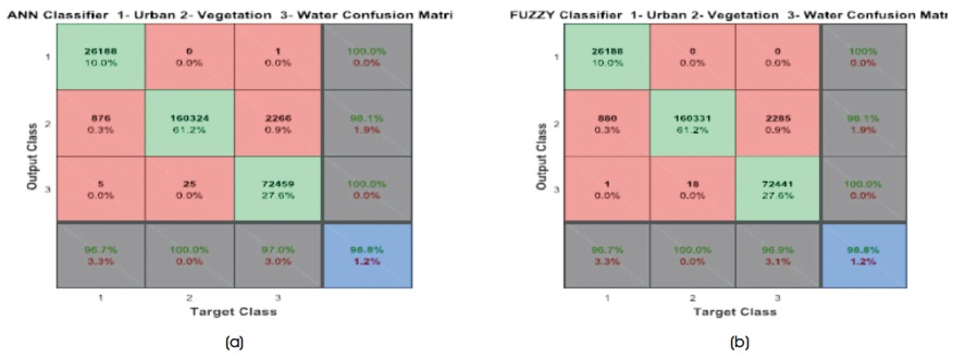
Figure 16. Confusion Matrix (a) ANN (b) Fuzzy
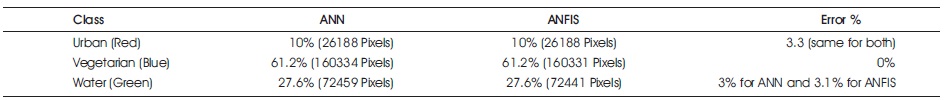
Table 1. Confusion Matrix ANN and ANFIS
The ANN classifier has shown slightly better results as compared to fuzzy classifier; however the simulations show that fuzzy classifier like ANFIS are at par with the ANN. Using both techniques, we successfully classified raw SAR dataset image upto 98.6 % with a minimal error of 1.2%.
SAR is an all weather imaging tool which takes the advantages of a moving platform to synthesize a large antenna aperture to produce fine resolution images. For understanding the physics and signal processing of SAR, the paper focused on range imaging and cross-range imaging which are the building blocks for SAR imaginary. In the range imaging section, LFM chirp signal found to be producing the finest resolution images. The image classified in RGB, representing features like urban, vegetation and water has been achieved. The percentage classification of each feature pixel in the image has been presented using confusion matrix.