(1)
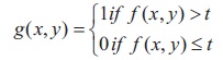
Image binarization is the process of representing an image pixel in binary format by assigning a value to the pixel as either 0 or 1. Before conversion to binary, the image can be in either gray-scale having pixel value between 0 to 255 or color, i.e., a pixel having value between 0 to 255 for each of the red, green, blue (RGB) channels separately. The method through which this conversion is implemented over an image is called as the binarization method. This paper reviews the methodology, contributions, advantages, and disadvantages of the existing studies on binarization methods. Further, the paper also highlights the problems in image processing with the scope for future enhancements.
Image processing is a broad concept that includes various techniques used in a wide range of applications. Binarization of an image is a direct and frequently used technique in image processing. A generalized binarization method of adjusting gray-scale image contrast irrespective of the document types has been proposed by Feng and Tan (2004). A thresholding technique for obtaining a monochromatic image (binarized) from a given gray-scale image of old documents is proposed in Mello et al. (2008). A broad survey of image processing from the industrial perspective has been given, though optical character recognition (OCR) technology has been available since the 1950s, both recognition hardware and computing power had drawbacks in the first two decades (Fujisawa, 2008).
In Badekas and Papamarkos (2007) preliminary binarization is obtained using a high threshold and the Canny edge detection algorithm (Canny, 1986). The initial results were refined using a binary image obtained with a low threshold. For images with low contrast, noise, and non-uniform illumination, this double-thresholding method is more effective than the classical methods. However sparingly, using entropy-based thresholding method achieved a reduction to 12% in image size, which in turn speed-up further processing.
In Kittler and Illingworth (1986), local thresholding is employed to detect casting and welding defects in machinery images and to separate the foreground and background in text and non-text regions in document images, respectively. Algorithms to handle the challenges in text segmentation of the images having complex backgrounds are discussed (Cavalcanti et al., 2006; Gatos et al., 2004; Oh et al., 2005). In Feng and Tan (2004), a local threshold value for binarization in low-resolution text is obtained with windows containing two consecutive letters. The frequency distribution in gray-scale values of image pixels is plotted as a histogram. Vertical and horizontal projection profiles of the documents image are considered during the binarization process. Valleys observed in the histogram give clues for selecting suitable threshold(s) value (Gonzalez & Woods, 2002; Sonka et al., 2007).
Ideally, a document having black letters on white background or viceversa will have a bimodal histogram (two peaks, one for the background and one for the foreground) of its image. While unimodal histograms (one peak) are observed in images when the text and background have similar intensities, as in the case of stone inscriptions. A multimodal histogram (several peaks) is observed for multi-colored text document. Thus, multimodal histogram generate multiple candidates for thresholds. Then, finding a pixel-wise threshold value to separate the text from non-text region becomes difficult (Jain, 1989; Russ, 2007). Interestingly, in many cases, the selected threshold value is based upon manual observations of the valley region(s), and then adjusted by trial and error to a value that works well (Russ, 2007).
For a global threshold value, t, g(x,y), is a thresholded image of a test image, f(x,y) (Niblack, 1986; Rosenfeld & Kak, 1982). The pixels are labeled either 1 or 0 representing the foreground or background. Suppose g(x,y), is a thresholded image of a test image, f(x,y), for a global threshold value, t. The pixel value in g(x,y) is equal to 1, if f(x,y) > t, and 0, otherwise.(Niblack, 1986; Rosenfeld & Kak, 1982). Figure 1 shows the histogram plots. Figure 1(a) shows the Brahmi script image on rock and its histogram in Figure 1(b). Figure 1(c) shows Grantha script image on palm leaf and its histogram is shown in Figure 1(d). In Figure 1(b), the unimodal histogram of the image suggests a single threshold value. The thresholding of an image is given by,
The pixels that are labeled either 1 or 0 corresponds to foreground or background respectively. Thus, thresholding converts a gray-scale image to a binary image by transforming all pixels value to either 1 or 0 such that above or equal to and below the threshold value, respectively (Gonzalez & Woods, 2002; Jain, 1989; MATLAB, 2011). Mostly, for a global threshold, the value of t, is arbitrarily chosen from a certain range of values for t and image details are observed precisely for the selected value (Gonzalez & Woods, 2002). In the same concept, for a single threshold in Figure 1(d) has two values for the image in Figure 1(c). Thus, the thresholding of an image is given by,
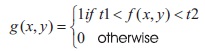
The bimodal histogram predicts two threshold values t1 and t2. If the image pixel value lies between t1 and t2 then it corresponds to 1, or otherwise it is 0 (Gonzalez & Woods, 2002; Niblack, 1986).
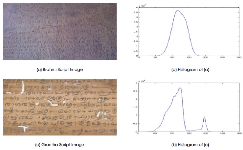
Figure 1. Two Histogram Plots with Single and Double Modes for Threshold Estimate
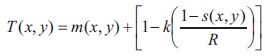
The histogram-based method fails when there is less difference between foreground and background intensities. The reason is that the valley between two peaks is not deep, so the histogram tends to a unimodal distribution. This problem is solved with a local thresholding method proposed by Niblack (1986) and Saxena (2019). Here, the threshold value is based on the mean and standard deviation of pixel intensities in a local window. The threshold for Niblack method is given by,
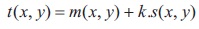
where m(x, y) and s(x, y) are the local mean and standard deviation, and k is a document-dependent manually selected parameter (Niblack used 0.2 for dark foreground and 0.2 for dark background). A large value of k adds extra pixels to foreground area which makes the text unreadable, while a small value of k reduces foreground area resulting in broken and incomplete characters (in a document having text and non-text regions). The main disadvantage of this method is that it produces a large amount of background noise, increasing the foreground region. This problem is solved in Sauvola and Pietikäinen (2000) by the thresholding formula,
where R is the dynamic range of the standard deviation s(x, y) and k takes positive values. This formula has the effect of amplifying the contribution of standard distribution in an adaptive manner. Hence, satisfactory results were obtained for 8-bit images when R is 128 and k is equal to 0.5. A large value of R (close to 255) produces dark background, thus reducing the foreground region. Sauvola's method is better than Otsu (1979) and Niblack (1986) methods but still there are some regions in image with pixels having background noise, as shown in Figure 2.
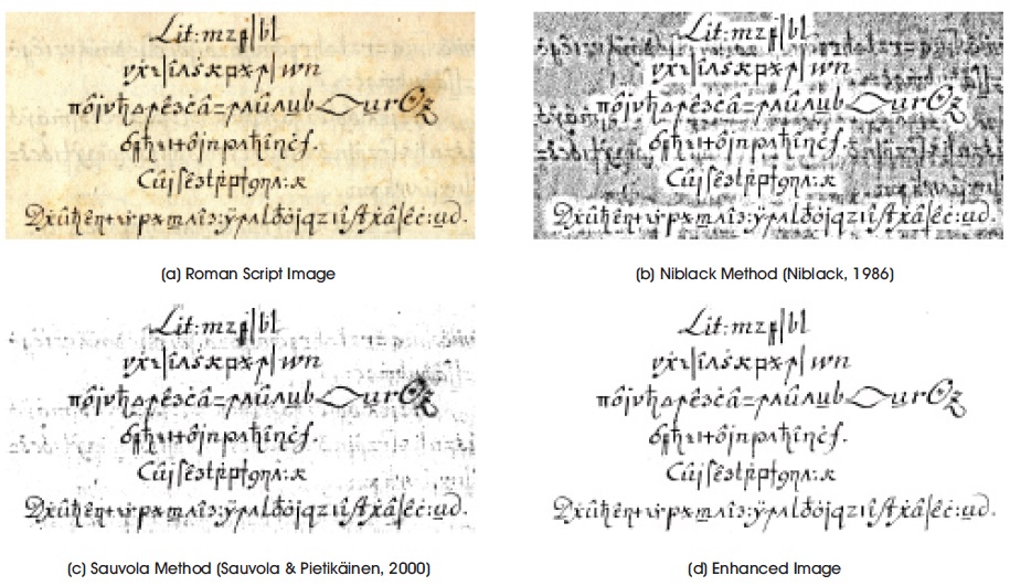
Figure 2. Result of Niblack's and Sauvola's Methods (Saxena, 2014)
However, in a two-stage thresholding technique based on fuzzy approach (Solihin & Leedham, 1999), first the image is separated into three regions: the foreground, the background and a fuzzy region with pixel intensities falling in between. The final threshold is found in the second stage after taking into account the distribution of intensities due to the handwriting device, e.g., a pencil has lighter intensity (lesser contrast) and more distribution of intensities than a ballpoint pen, whereas a felt-tipped pen has higher intensity (greater contrast) and less distribution of intensities. The Native Integral Ratio (NIR) helps separate the foreground and background from the fuzzy regions, while a new technique (Solihin & Leedham, 1999) called quadratic integral ratio (QIR) reduces local fluctuations that are introduced by NIR.
Also, the method described in Yang and Yan (2000) uses run-length histogram of grayscale values in degraded document images. First, the clustering and connection characteristics of a character stroke are analyzed from the run length histogram for selected image regions and various inhomogeneous gray-scale backgrounds. Then, a logical thresholding method is used to extract the binary image adaptively from the document image with complex and inhomogeneous background. It can adjust the size of the window and thresholding level adaptively according to the local run-length histogram and the local gray-scale in homogeneity. This method can threshold poor quality gray-scale document images automatically without needing any prior knowledge of the document image and manual fine-tuning of parameters.
When histogram-based thresholding techniques fail to satisfactorily separate the text (that is, a global threshold does not work for the whole image), optimal threshold values suited to different regions in the image are generated through adaptive binarization (Batenburg & Sijbers, 2009; Gatos, 2006).
Adaptive binarization is employed for segmentation, noise reduction, and document analysis (Baird, 2004), optical character recognition (Casey & Lecolinet, 1996; Plamondon & Srihari, 2000; Trier et al., 1996), imaging 2-d planes of 3-d objects (Leedham et al., 2003) and for the specific purpose of manuscript digitization, restoration and enhancement (Kavallieratou & Antonopoulou, 2005; Perantonis et al., 2004, Sparavigna, 2009). A comparison and evaluation of different adaptive binarization techniques is given (Blayvas et al., 2006; Duda et al., 2001; Trier & Jain, 1995; Trier & Taxt, 1995). A short survey by Kefali et al. (2010) presents a comparison of global and local thresholding methods for binarization of old Arabic documents image enhancement. Several binarization methods are compared on the basis of relative area error (RAE), mis-classification error (ME), modified Hausdorff distance (MHD) (Sezgin & Sankur, 2004). An adaptive thresholding method is proposed in Sauvola and Pietikäinen (2000) to enhance degraded documents images, while the method in Gatos et al. (2004) interpolates neighboring background intensities for background surface estimation as shown in Figure 3.
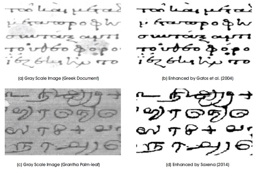
Figure 3. Greek and Grantha Manuscript Gray-scale (Saxena, 2014).
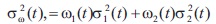
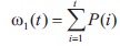
The global threshold method proposed by Otsu (Otsu, 1979) is based on histogram processing, such that histogram interpretation reveals a separation of pixels into two classes for foreground and background. The threshold selection tends to minimize the weighted within-class variance σ2ω(t) given by Equation (5):
Here the class probabilities are calculated by:
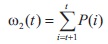
And the class means are calculated by:
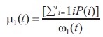
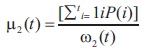
Finally, the individual class variances are calculated by:
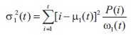
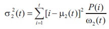
where 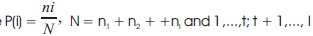 are gray levels. Hence, the total variance is calculated by adding within-class and between class variances, which is represented by Equation (12):
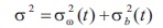
where
Here, σ2 is a constant value irrespective of the threshold value, however minimizing σ2ω(t), weighted within-class variance or maximizing σ2b(t) between-class variance leads to threshold value which lies between 0 to 255.
The threshold in Kittler and Illingworth (1986) is calculated by minimizing the criterion function.
where h(z): z = 0, 1,..., Z -1 the normalized histogram, c(z, ) is cost function, τ, the threshold based on hypotheses H0 and H1 such that,

for k = 1, 2,..., N.
The threshold calculation by solving Laplace Equation in Yanowitz and Bruckstein (1989) is defined by Equation (16):
where P(x, y) is the potential surfaces for (x, y) as the data points, is to estimate the gray-level values to interpolate the threshold surface, which smoothens the image and calculates the gradient magnitude.
An input sensitive thresholding algorithm defined in Yosef (2005) for binary image using Equation (17):
where f, is the gray-scale image and Tf, is the global threshold, defined by:
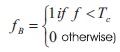
where TC, is the mean gray-scale value of CB (set of pixels belonging to contours of components in fB). Further a reference image is obtained by calculating a local threshold by:
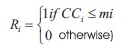
where i = 1,...,N, CCi is the connected component, mp, is the mean gray-scale value of pixels belonging to CCi.
The mean gradient technique proposed by Leedham et al. (2003) is defined by:
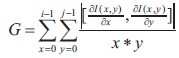
where I(x, y) is the intensity image. Since, the gradient is sensitive to noise, adding a pre-condition referred to Constant R, improves in selecting a threshold level, such that:
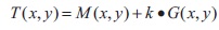
else
where k = -1:5, R = 40; parameters M(x, y) and G(x, y) are the local mean and local mean-gradient calculated in a window centered at pixel (x; y), for Constant=max|gray value|-min|gray value| in a window.
The local threshold calculation method in Feng and Tan (2004) is defined by:

where  α1, γ, k1 and k2 are the positive constants, m(x, y) is the mean, s(x, y) is the standard deviation, M is the minimum gray value, and Rs is the s dynamic range of gray-value standard deviation. The value of γ is fixed to 2 and the values of other factors like 1, k1, and k2 are in the ranges of 0:1 - 0:2, 0:15 - 0:25, and 0:01 1 2 - 0:05 respectively.
The modified waterfall model for threshold calculation in Oh et al. (2005) is given by:

where I'(x, y) represents the water-filled terrain, G(j, k) denotes the 3 x 3 Gaussian mask with a variance of one, and parameter controls the amount of water-filled into a local valley (α=2), water falls at (xi, yi) and reaches the lowest position (xL, yL).
It is an entropy based threshold calculation method proposed by Mello et al. (2008), given by:
there are n possible symbols, s, with probability p(s), where entropy is measured in bits/symbols, which maximizes the function by:
where Hb and Hw are the entropies of black and white pixels bounded by threshold t, for Hb: 0 to t and Hw: t + 1 to 255. This method introduced two multiplicative constants mw and mb, which are related to class of documents given by:
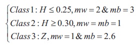
where Z = 0:25 < H < 0:30, threshold th is given by
each pixel i with color graylevel[i] in scanned image is turned to white, if 
For the documents having varying background contrast, there is a suppression method detailed in Su et al. (2010) which uses local image maximum and minimum defined as:
where fmax(x, y) and fmin(x, y) refer to the maximum and minimum image intensities within a local neighborhood window of size 3 x 3. The term ϵ, is a positive but infinitely small number added when local maximum equals to 0. The thresholding equation is defined as:
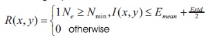
where is input 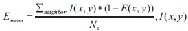 document image,
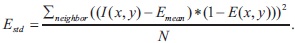
Emean and Estd are the mean and the standard deviation of the image intensity of the detected high contrast image pixels. (x,y) denotes the pixel position, Ne is the number of high contrast pixel in window, and Nmin is the minimum number of high contrast pixels.
The method in Blayvas et al. (2006) found an adaptive threshold surface by interpolation of the image gray levels at points where the image gradient is high, which is given by:
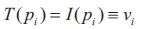
where pi = xi, yi and vi = I(xi, yi) denotes the ith support point. The unit step source function is defined by:
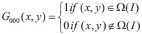
here W(I) = [0, 1]2 denotes the set of all image points. The shifting is given by Equation:
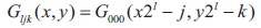
where l = 0,..., log2(N) is a scale factor and j; kϵ0,..., 2i - 1 are spatial shifts. Hence, the threshold surface is given by:
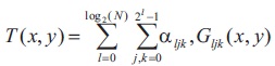
The thresholding method in Saxena (2014) is defined by:
where 'k' lies between [-0:5 to +0:5], the constant of proportionality valued at 1/4 gives satisfactory results with Grantha and other manuscript images. 'k' does not affect much, since the value of 2(k+1) s(x, y) will always be a positive value. The factor  lead towards the improvement in terms of preserving the strokes width, maintaining the shape and connectivity, which is solely needed for recognition purposes.
This section discusses the datasets used by the respective methods explored in Section 2. The research work in Otsu (1979) used several images of size 64 x 64 pixels. Images include layout structures, character or symbols, and the cell, all were in gray-scale.
The manuscript restoration work in Yosef (2005) used thirty Hebrew calligraphy manuscripts from 14th to 16th century. The size these manuscripts varies from 2000 x 1000 to 8000 x 6000 pixels, and roughly these were split into 3000 x 2000 pixels. Specifically, each split part contained an average of 200 characters, with an approximate size of 80 x 80 pixels. The method in Saxena (2014) tested manuscript images on different media having different scripts: Palm leaf (Grantha), rock (Brahmi), and paper (Modi, Newari, Persian and Roman), and DIBCO datasets. The dataset in Leedham et al. (2003) used the set of ten images of historical handwritten documents, cheques, forms and newspapers.
The binarization method in Feng and Tan (2004) tested eight set of document images in various sizes and having uneven illumination, low-contrast, and random noises. Also, this method applied a median filter of size 5 x 5 in order to remove additional noise. The constant terms namely, γ, α1, k1, and k2 for test set are fixed to 2, 0.12, 0.25, and 0.04 respectively. Hence, to reduce computational complexity, the local threshold at the centers of the primary local windows are bilinearly interpolated to obtain the threshold values for all the pixels.
The experimental dataset without ground-truth data is discussed in Oh et al. (2005). However, the experimented data consists of ten document images obtained by a scanner with 200 dpi having a size of 256 x 256 pixels with 8- bit gray-levels. The threshold computation time of 3.2 seconds per image implemented through C++ is obtained in Mello et al. (2008). Further, the test set comprised of five hundred images with at least 200 dpi in JPEG format. The binarization method in Su et al. (2010) tested the dataset from Document Image Binarization Contest (DIBCO) 20091, which is available online.
Without specifying the exact number of images the method in Kittler and Illingworth (1986) experimented various images of objects and structures with different gray levels. Interestingly, the artificially constructed gray-scale images having prominent white noise and uneven background illumination are processed in Yanowitz and Bruckstein (1989). In addition, this work extended experimenting these images having added narrow-band noise in their spoiled versions. Another work in Blayvas (2006) on artificial images generated four black and white images by simulating non-uniform illumination of the black and white pattern. Further, this work proposed a quantitative measure of error of the binarization method, calculated error as normalized L2 distance between binarized and original black and white image.
This section presents the discussion on the application of binarization methods for documents images. The global thresholding method in Otsu (1979) automatically selects a threshold from the gray level histogram distribution of pixels. This method finds between-class variance from gray-scale values distinguished as group of foreground and background pixels. Hence, the method is supposed to be global in nature as it selects a single value for every pixel of the image. In results, this method is unable to preserve minute details in the image, such as connectivity of the characters.
The objects in artificially constructed gray-scale images are clearly detectable through Kittler and Illingworth (1986). Further, this method works only on the nicely bimodal histogram (observable foreground and background). The evaluation of binarization method in Yanowitz and Bruckstein (1989) performed better than Chow-Kaneko detecting bi-modality of partial histograms and Rosenfeld- Nakagawa processes failed to detect faint objects. In addition, this work claims that the proposed model is comparable with human performance.
The efficiency in correctly segmenting characters from the document image is up to 94% (Yosef, 2005). Additionally, the efficiency in segmentation increased to 98% in a substantial set. Further, as a drawback the computational complexity is reduced for the brighter images. And the generalization of this approach is left for the future scope. The essence of the proposed method in Leedham et al. (2003) is that it processed difficult gray-scale document images having varying pixel intensities. However, the method failed to threshold double-side affected (or bleedthrough) and noisy background document images.
The character recognition rate for machine-printed characters through Feng and Tan (2004) has been up to 90.8%. Further, this work claimed the robustness of the binarization method to uneven illumination. The suppression of noises in non-text regions and completeness of binarized text characters is evident through binarization results. However, there is no evidence of testing on handwritten character images. The proposed method in Oh et al. (2005) proved the effectiveness of the waterfall model through visual observation only. Further, the method surpassed in comparison of processing time of original and proposed waterfall model.
The problem with the documents that are written both sides is the essence of the method in Mello et al. (2008). Further, this work observed that the written documents are 10% in ink (text regions) and 90% in paper (non-text regions). For processing, the size of the images has been reduced from 500 KB to 40 KB, which dropped the processing time 97% of the actual time. In Su et al. (2010), the observation identified different types of document degradation such as uneven illumination and document smear. For future studies, it proposed that error may arise if the background of the degraded document images contains a certain amount of pixels that are dense and at the same time have a fairly high image contrast.
The work in Blayvas et al. (2006) claimed lower computational complexity and smoothness of the proposed binarization method. In addition, this work claimed faster yield of binarized images and better noise robustness. However, there has been no comparison of the proposed method with Sauvola's binarization method. The readability of text up to 66.27%, 92.15%, 97.90%, 56.23%, 78.62%, and 98.91% for palm leaf, and paper manuscripts is obtained in Saxena (2014). Additionally, this work showed the effectiveness of the window size (33–1515) is observable in terms of processing time. Further, it stated that, smaller the window size the more time it takes in processing.
Binarization of an image is a direct and frequently used technique in image processing. Many methods in the literature have been shown to be effective in handling the complexity of binarization. The histogram-based method fails when there is less difference between foreground and background intensities. Thresholding converts a gray-scale image to a binary image by transforming all pixels value to either 1 or 0 such that above or equal to and below the threshold value, respectively. Some algorithms need extensive manual intervention, which make the methods less attractive. Adaptive binarization is employed for segmentation, noise reduction, and document analysis, optical character recognition, imaging 2-D planes of 3-D objects, and for the specific purpose of manuscript digitization, restoration and enhancement. Most of them are designed for specific applications, and so are lack generalization. This paper contains a summary of binarization and thresholding methods, their implementation, usability and challenges.