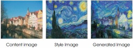
Figure 1. Neural Style Transfer
By composing a complex interplay between the content and style of an image, humanity has mastered the ability to create unique visual experience in fine art, particularly painting. Transfer of the artistic style is a problem in which image style is transformed into image content and generates image stylization. Style transformation can be applied over the entire video sequence by adding image style to video. We use perceptual loss functions to train feed-forward neural network and extract high-level features from the trained networks. We show the effects of image style transfer and video style transfer, through training feed forward network. Our network delivers faster results when compared with Gatys proposed optimization-based method. Resnet is added to the network as an improvisation to transformation network. Pruned Resnet is used, and it gives high computation speed, less size of memory and good performance.
Style transfer is a method of changing the style of an image while still preserving its content. There are different applications in the last decade that style images in a way that gives the illusion of being like paintings. There are two input images used to generate a new image known as stylized image, especially image content and image style. The generated image will have both the content and the style. These two pictures are performed without overlapping. Numerous studies and different types of techniques exist that automatically turn photos into digital artwork. Non- Photorealistic Algorithms are designed with limitations for stylization rendering. They are made for specific styles only, and cannot be extended to other styles. Style transfer is being studied as a generalized texture problem from source within the computer vision community. Hertzmann et al. (2001) suggested a generalized concept transfer platform called "Image Analogies”. There are several drawbacks to these methods. We only use low-level image functionality, and failed to effectively capture image structure. Gatys first studied the convolutional neural network with a view to reproducing famous painting styles on natural images. Gatys have proposed a new field called Neural Style Transfer (NST) referring to Figure 1. NST is a method of using convolutional neural networks to create images of content in different styles. Many common problems can be considered as processing images in which the network gathers and converts any of the image data into an image output.
Figure 1. Neural Style Transfer
Many common problems can be considered as processing images in which the network gathers and converts any of the image data into an image output. Methods of image processing involve denoising, high resolution, filtering and data distortion (noise, low-resolution or gray) leading to a high-quality color image. Semantic segmentation and depth estimation are computer vision examples, where the input is a color image, and conceptual or semantic scene information is represented by the image output. One way to handle image processing tasks is to design a convolutional neural network that provides a pixel. Loss approach for the evaluation of the difference between the images and the ground-truth. In specific, Cheng et al. (2015) for coloration, Long et al. (2015) and Noh et al. (2015) for the segmentation and Eigen et al. (2014) for the normal prediction of depth and surface, and Dong et al. (2015) used for super resolution with colorization. Such methods operate through training periods and then require the improvement of the qualified network. Furthermore, no noticeable differences between images from the displays and from the field are observed by the losses per pixel use in those techniques. Taking two identical images in comparison, for example, to the images calculated by a loss per pixel that are compensated for perceptuality. At the same time, the recent research has shown that images of high quality can be generated with perceptual loss functions, not on the basis of differences between pixel and neural convolutional networks but on the basis of the differences between high image representations. Pictures are generated to reduce the loss function. This technique refers to the inversion function of feature visualization, and features added by Mahendran and Vedaldi (2015) and Simonyan et al. (2013). Gatys et al. (2015) style transfer are strategies that yield high-quality images, but are slower because deduction requires inferior resolution of the optimization problem.
The article uses the benefits of these two methods. Transformation networks are trained for image processing purposes, but we train our networks with high-level perceptual loss functions from a trained loss network, instead of using per-pixel loss functions that depend only on low-level pixel details. During training, perceptive losses are more stable than losses per pixel during image comparisons and transformation networks function in real time. We are working on two tasks: Image style transfer and Video style transfer. A feed forward network in Figure 2 is designed to solve the problem of optimization much faster than previous approaches.

Figure 2. Network Architecture
Feed Forward Image Transformation: Over the last years a large range of input image transformation tasks have been solved by training deep, convolutional neural networks with per-pixel loss functions. Semantic segmentation techniques create complex labels for scenes to train with a lack of per-pixel classification by running a network on a regular, pixel CRF image in combination with the rest of the network. The transformation architecture in the network is inspired by Long et al. (2015) and Eigen et al. (2014) using the sampling of the network to minimize the spatial scale of function maps, followed by a sampling of the network to provide the final image.
In turn, new depth and standard surface estimate procedures use convolutional feed-forward network trained in a pixels regression or loss classification to transform the color input image into natural meaningful output image. Such approaches are per pixel loss by the penalization of image gradients or the use of a loss layer of CRF in order to improve local accuracy. The feed forward is trained to transform gray scale images into colors by per pixel loss.
In Gatys et al. (2015) texture synthesis techniques, related techniques have been previously used in order to transform art form, integrate contents of an image from another, as well as reducing losses in feature reconstruction and loss of style often based on pretrained convolutional network features. Our solution yields high quality results but is informative and expensive, because for every stage of the optimization problem a forward and backward transformation by the pre-trained network is necessary. The feed network is designed to easily identify solutions to their optimization problems. The image processing network for transforming input images in the output is trained. In Figure 3 we are using an image classification pretrained loss network that describes functions of perceptual loss that quantify observable image differences in content and style. The network of losses remains stable throughout the training phase.
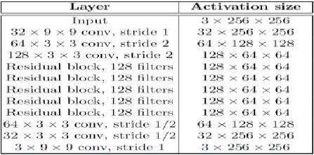
Figure 3. ResNet Architecture used for Style Transfer
Many articles have used optimisation to generate images based on high level properties from a convolutional network in which the result is visible. Images may be created within eligible networks in order to optimize classification results or individual features to understand encoded functions. Similar optimization approaches can also be used to create high level images.
In this paper, in feed forward networks we use perceptive loss functions (Johnson et al., 2016), rather than using pixel loss functions that are trained for image transformation work.
Comparing two images, depending on their pixel values, and if two images rely on just one pixel, and are perceptively the same but different from each other, then the loss functions per pixel would render them different.
Semantic differences in images and estimation of highlevel detection functions. We are able to visualize images using a pre-trained loss network, thereby allowing visual loss itself highly complex neural networks. All the results on the 2014 Microsoft COCO dataset are pre-trained in the VGG- 16 layer network.
Instead of activating the output image pixels y ̂= fx (x) to exactly match the target image y pixels, we let them have specific feature representations to those defined by the network of losses f. Let ∅j (x) be network j layer activations ∅ if Image x is processed, if j is a convolution layer, ∅j (x) will be processed.
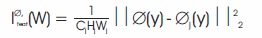
Wj shape function map for Wj Reconstruction loss feature is (Squared, Standardized) Euclidean distance between feature representations as in Equation (1).
Finding an image y minimizes the loss of the feature reconstruction of the early layer. It is practically inseparable from y. The image quality and the overall spatial structure are maintained when we reconstruct from higher levels, but colour, texture are not the same format. Using a reconstruction loss function to train our networks of image transformation helps to make the resulting image perceptible but does not require them to fit exactly.
The loss of the reconstruction of feature penalizes the image output if it deviates in consistency from the target. Colors, textures, shapes etc form the basis of style penalization variations.
Two other loss functions depend on low-level pixel information rather than perceptive losses.
The pixel loss is the uniform difference between the output y and the y source. This can be used when matching target ground-truth with network.
Follow the inversion function for the complete difference regularizer to achieve spatial smoothness in the output image. We train style transfer feed networks that try to solve Gatys et al. (2015) problem of optimization.
In architecture, two neural networks are needed to successfully train a generative style transfer model. The first network is called the transformation network and is used to create new images based on input images. And the second network is a network of losses used for evaluating the images generated and for calculating the loss. Then loss function is used to optimize the transformation network to generate better images. The transformation network is known as f (x). The network can be fed an input image x w and transferred through the network y=fw (x) to an output image y. This network is trained with stochastic gradient descent to minimize a weighted combination of the loss functions. The total loss can be defined as a linear combination of both the loss of the feature reconstruction and the loss of the style reconstruction by reducing the overall loss, a model well trained with weights W*.
As a transformation network that can produce stylized images is already defined, next a loss network that is used to represent multiple loss functions to evaluate the generated images and use the loss to optimize the transformation network based on stochastic gradient downward. A deep, convolutional neural network is used to measure the style and content differences between the generated image and the target image for image classification on ImageNet dataset. Recent research has shown that deep convolutional neural networks can encode the details about the texture and high-level content in the function maps. Based on this analysis, a content reconstruction loss is defined as icontent within the loss network as well as a style reconstruction loss with its weighted sum to measure the total difference between the stylized image and the image to be obtained. The transformation network is trained with the same pretrained network of losses for every model, which means the network of losses should remain the same during the training phase.
The images with similar features should have similar feature representations computed by the network of deep CNN tℎ losses. ∅j (x) is used to represent the loss network in J layer for image x processing and the content image that should be Cj*H*Wj. The Euclidean distance is then used to reflect the loss of the content reconstruction. A generated image from the transformation network that can reduce the loss of content reconstruction in order to get the half ∅j (y) that has similar high-level semantic features but does not have to be the same with the target image information. In the Style Reconstruction Loss, the images produced would have the same texture synthesis with the target image type, so the type variations are penalized with the loss of reconstruction quality. More specifically, the work found that the Gram Matrix used the difference in texture between the two images from the feature map. Similarly, with a feature map ∅j (x) in the jth layer of the shape Cj X Hj, the Gram matrix is defined as G∅ (x) to be a matrix Cj X Cj.
The image that is stylized may contain low level noise. The presence and information of the noise indicates this is caused by the Convolutional Neural Network filters. Full denoising variance is a method for eliminating noise from the image processing.
To test the efficiency of this method, the image recognition tasks need to be conducted with the images that are stylized. When transforming images, the programs or algorithms need to generate the most logical categories of objects for each given image. The algorithm performance is usually measured based on whether the predicted category matches the image ground-truth label. If an input image is taken from multiple categories, an algorithm overall output is the average score of all test images. Once the transformation network that can generate the stylized images is trained, a larger dataset is applied to the training dataset.
The Res Network (ResNet) is a Convolutional Neural Network (CNN) architecture, designed to adapt hundreds or thousands of layers. Even though previous CNN architectures had an additional layer efficiency decline, ResNet can add several layers with good output. The continuous multiplication of each additional layer decreases the gradient until it stops, satures or even degrades the output as too many layers occur.
ResNet solution is "shortcut identity links". ResNet stacks identity mappings, the layers which cannot do anything at the first point. Originally, skipping compresses the network into multiple layers allow to understanding faster. Instead, all layers are expanded until the network trains again and the "residual" parts of the network are gradually exploring the feature space in the source picture. Uses a specific method of identity mapping with separate directions and their outputs merged through the introduction of the layered identity layers. ResNet adds a new "cardinal" hyper parameter that sets the number of paths in a line. ResNet is a scope of the issue of "vanishing gradients". The reverse propagation process of neural networks, which depends on gradient descent, decreases the weight loss function and reduces it.
COCO is a vast image dataset designed for object identification, segmentation, personal keypoint identification, object segmentation and caption generation. This package provides COCO annotations for the Matlab, Python, and Lua APIs that help load, read, and visualize. The Microsoft COCO dataset 2017 is used for the transition of information. Images input are in jpg format (Joint Photographic Group).
MPI Sintel Dataset-23 training scenes with a resolution of 1024 X 436 pixel by scene in 20-50 frames. It also outperforms all the optical flow methods reported on the Sintel MPI final transfer, running at approximately 35 fps on images with sintel resolution. MPI Sintel Dataset is used for video style transfer implementations. The training scenes will be stylized, combining all the frames to form a video. Refer to the sintel video from the training scene taken from Table 4.
Videvo dataset consists of many video groups. It consists of different video resolutions (low resolution, high resolution, HD, 4K) which can be used to stylize the video. In this paper two videos with two different resolutions are taken from the Videvo (Table 7) showing all the properties of the videos. This video will be taken as a content video, first dividing the video into frames by frame rate. Then the style image is added to all frames, then all the stylized frames are combined to reduce the error loss by using the loss function, the stylized video is created as output. You can save the stylized video in the required format. The present approach requires very less time to convert stylized video compared to the previous approaches.
We perform experiments on image style transfer and video style transfer. Feed forward network gives the much faster result when compared to the other methods.
Our style transfer network is trained on the Microsoft COCO dataset. 80k training images are resized to 256 x 256 and batch size 4 is taken to train our network. Adam optimizer is used for optimization. Our implementation uses Torch and cuDNN, training takes roughly 4.8 hours on Tesla P4 GPU.
For training the transformation network the required packages are mentioned in Table 1. The training can be done by using Google Colab, Anaconda (windows, ubuntu).
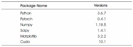
Table 1. Package Versions Used for Training in Google Colab
For training the transformation network GPU is required. Because running the style transfer technique on CPU takes very long time. GPU can be used by default or CUDA, or by using Google Collaboratory. The hardware versions mentioned in Table 2 is used in Google Colab. Runtime mentioned in Table 2 and virtual Machine runtime in Google Colab. After 12 hours the VM runtime gets disconnected.
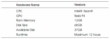
Table 2. Hardware Versions Used for Training in Google Colab
Training the transformation network required some basic parameters mentioned in Table 3. Based on these parameters the training results will vary. The dataset used for the training is Microsoft COCO train 2014 which consist of 20k training images. The Batch size can be changed based on the training dataset. If the dataset is large the Batch size can be increased. The value of epoch also can be increased.
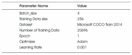
Table 3. Basic Parameters for Training
Training dataset was experimented with different parameter values to get the better results and to reduce error loss. Microsoft COCO train 2014 dataset was trained for the experiments.
Experiment 1: Training COCO train 2014 dataset with content weight=17, style weight=50 (Table 4).
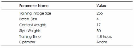
Table 4. Above Experiments Results Comparison in Different Iterations with Images
Training the transformation network with the content weight =17, style weight=50, with batch size 4, by using adam optimizer for 256 size images the training time was 4.8 hours which is much faster than the previous style transfer approaches. Figure 4 gives the information about the results obtained by training. It gives the loss history of the content, style, and total variation loss.
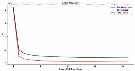
Figure 4. Total Loss Graph of Experiment 1
Experiment 2: Training COCO train 2014 dataset with content weight=20, style weight=20 (Table 5).
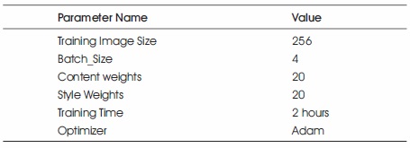
Table 5. Details of Experiment 2
Training the transformation network with the content weight =20, style weight=20, with batch size 4, by using adam optimizer for 256 size images. The training time was 2 hours which is faster when compared to the content weight=17, style weight=50. Figure 5 gives the information about the results obtained by training. It gives the loss history of the content loss, style loss, and total variation loss.
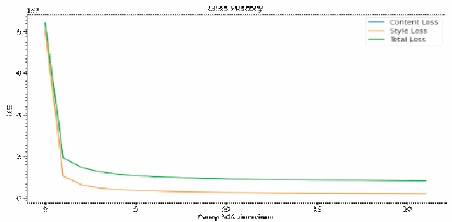
Figure 5. Total Loss Graph of Experiment 2
Experiment 3: Training COCO train 2014 dataset with content weight=50, style weight=50 (Table 6).
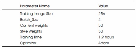
Table 6. Details of Experiment 3
Training the transformation network with the content weight =50, style weight=50, with batch size 4, by using adam optimizer for 256 size images, the training time was 2 hours which is faster when compared to the content weight=17, style weight=50. Figure 6 gives the information about the results obtained by training. It gives the loss history of the content loss, style loss, and total variation loss.
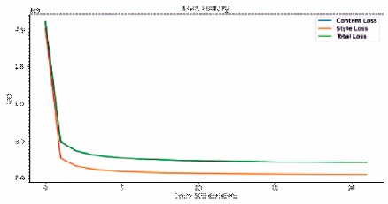
Figure 6. Total Loss Graph of Experiment 3
The Figure 7 gives the information about the results obtained by the experiment 1, experiment 2, and experiment 3. The train 2014 dataset consist of 20696 images which is dived by the batch size 4, with 1 epoch, by using the adam optimizer. The results has been taken from 4 iterations. The three experiment results will show the difference between the iterations and the experiments. The results shows how the style image is applied on the content images.
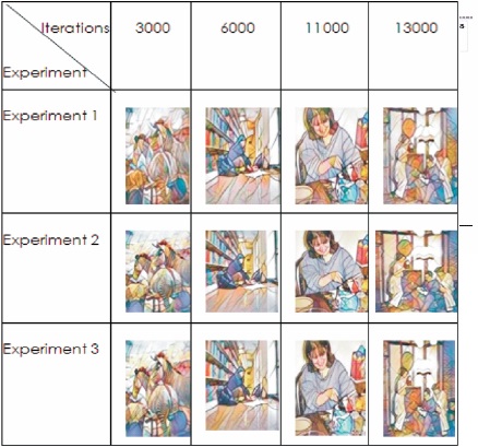
Figure 7. Comparison in Different Iterations with Images
The style transfer technique applied on the images with the size 256. This technique is implemented in transformation network.
Table 5 depicts that transformation network takes less than 2 seconds to transform the images with less error loss.
Image style is implemented in two methods and the runtime of our method is faster than the Gatys method explained in Table 6.
The mentioned frames in Figure 8 are samples of original video and the stylized video.
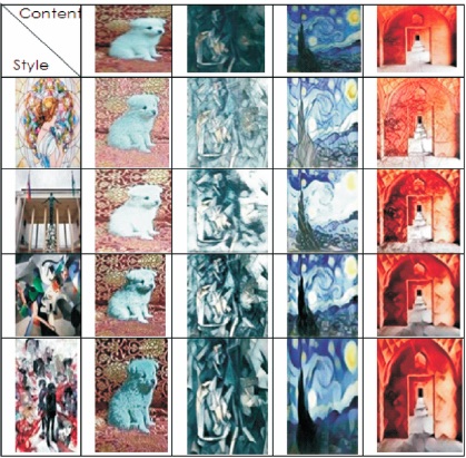
Figure 8. Style Transfer of Images
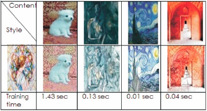
Figure 9. Frames of the Video
Three different videos have been taken, sintel, cat, rabbit are taken as a input videos with different resolutions. Refer to the Table 7 for the video properties.
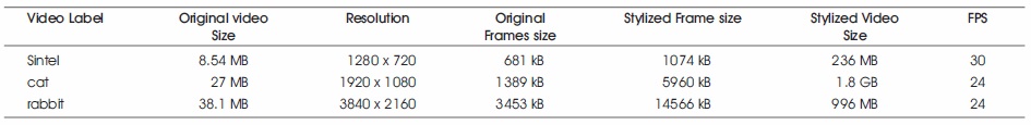
Table 7. Comparison of Different Video Properties
As the extension to the transformation network the ResNet is added as a layer. The network is pruned to minimize the network size which gives the result of fast training, with less memory occupation. The training time of the Transformation ResNet Network is faster than the Transformation Network. The content loss is less when dataset is trained with the Transformation ResNet Network. Table 9 shows the loss values mentioned in training time.
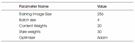
Table 8. Experimental Method for Image Transformation
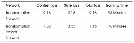
Table 9. Difference Between the Losses of Present Method and its Extension
Image style transfer and video style transfer can be implemented by using the image transformation method. The Previous approaches are implemented by using the neural style transfer algorithm which has optimization problem. To overcome the optimization problem, Johnson used perceptual loss function with image transformation network which works much faster than Gatys approach. Our Network is trained with different content-weight and style-weight which gives better performance by changing weights.
As the improvisation to the Transformation Network, ResNet was added as a layer. The advantage of the Pruned ResNet layer is speed computation, less memory size and high performance compared to the transformation network. When the transformer network and transformer ResNet network are trained transformer ResNet is faster. It needs to be improvised more to reduce more error loss. Comparing to all the previous approaches pruned ResNet network is more useful. This tiny ResNet model can be used by many style transfer applications for image and video styles. The pruned ResNet network is taken for the experimental purpose and it can be improvised based on the requirements.