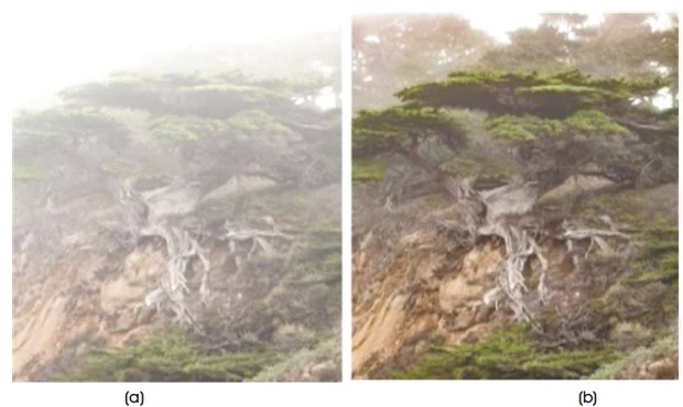
Figure 1. Color Attenuation (a) Hazy Image, (b) Dehazed Image
Haze removal is a serious problem while dealing with single image. In this paper, the authors have proposed a new simple and powerful method to dehaze an image called color attenuation prior. Here, a depth map of the image has to be created at first, from a previously created linear model under the novel prior. From this find the transmission map so as to retrieve the depth information clearly. Then the last step is scene radiance recovery from which it is possible to get the dehazed image. The scene radiance recovery is done by the using the difference between saturation and the brightness of pixels. The experimental results show that the proposed method is very efficient and has a advantage, that it can dehaze sky images too.
The outdoor images taken in the bad weather are usually comprised of fog or soot particles. The systems available now are not working properly as they are dependent on the reality of the input images and the presence of degraded or hazed images, leads to the need to improve dehazing techniques to rectify this problem. There are different techniques and these techniques are classified into two broad categorization, Multiple image processing technique and Single image processing technique. Usually, the processing for multiple images are difficult thus the processing for single image is mostly used nowadays. The authors have introduced a method to improve the contrast of image and helped in developing a cost function in frame work of Markov Random Field. The second method is used to increase scene visibility and then recover a hazeless or haze-free image constrasts. Previously dehazing was done for one image and then it is developed to work for many images (Tripathi & Mukhopadhyay, 2012). However, haze removal is actually demanding as it is based on the depth information of the haze (Schechner, Narasimhan, & Nayar, 2001). If the input is only one image then the case is under constrained. Various techniques have come up using multiple images. Considering images at different degrees of polarization helps to remove haze using polarization methods. For finding depth information there is a need of data from user input or from 3D models.
The haze removal using single image is more accepted strong priors are used for this. Considerable improvement is seen in dehazing a single image using physical techniques. By presuming that local contrast of haze-free image is better than hazy image, the researchers approached with a new technique for increasing local contrast based on Markov Random Field (MRF) that generates over saturated image. Fattal (2008) suggested a method to remove haze in an image by using the method of Independent Component Analysis (ICA). It is time consuming and cannot be used for gray scale images. He, Sun, and Tang (2011) detected the Dark Channel Prior algorithm (DCP) on non-sky patches. It is possible to visualize at least one color with very low intensity, which is almost equivalent to zero. In this method the haze free image can be recovered back making use of scattering model. This technique is useful, but the trouble is that it cannot be applied for sky patches and it is computationally very exhaustive, lots of other methods are now overcoming this technique. When many techniques were determined for haze removal of single image, it is a very complex problem (Zhu, Mai, & Shao, 2015; Preetham, Shirley, & Smits, 1999). The application of such method is very difficult to implement. To overcome all these problems the authors have introduced a new method in this paper called the haze removal using color attenuation prior. This is a very easy and effective method to dehaze image faster with less difficulty.
Demerits of Existing System
He, et al. (2011) found Dark Channel Prior (DCP) in non-sky images there will be at least one color channel that has some pixels whose intensities are low and somewhat equal to zero. In this method, the dehazing is done using atmospheric scattering model. It is an efficient model, but it cannot handle sky images and is comparatively computationally effective. Dark channel prior is actually used as a statistic for outdoor image haze removal.
It is very difficult to remove haze from an image in computer. Human brain can able to detect the hazy areas without the need of any additional information. The authors conducted a study on hazy images to make a prior for single hazy image. From their studies they came to know that brightness and saturation of the input hazy image differ with the concentration of haze. In an ordinary image for this research, the haze free regions have more saturation, the brightness here is moderate and the distinction between the saturation and brightness is almost zero. When haze comes into play, in the hazy image the saturation gets decreases and the color of the haze also decreases and the brightness gets increased. Here, it is difficult to identify the color of the image, and the difference value is also higher here (Schaul, Fredembach, & Süsstrunk, 2009; Xu, Liu, & Ji, 2009). The brightness and saturation difference vary greatly for hazy images.
The Figure 1 shows the haze removal in proposed method.
Figure 1. Color Attenuation (a) Hazy Image, (b) Dehazed Image
The color attenuation prior technique is very efficient for hazing single image. Initially a linear model to find the depth information is created and the parameters are found. Then a depth map from the depth information is generated. With the information from the depth map it is easy to evaluate the transmission and then restore the scene radiance by making use of atmospheric scattering model, thus the haze can be removed from the image.
This method overcomes all other algorithms used for dehazing when considering the efficiency. Five elements are mainly used for image dehazing, they are: Estimation of the depth information, estimation of transmission map, estimation of atmospheric light, scene radiance recovery and experimental result analysis. In the first element, when the haze dense is high the influence of the airlight will also increase. So, this helps us to estimate the difference between the brightness and saturation so as to find the concentration of haze in the image. The difference found here increases as the concentration of the haze increases. Here, there are two mechanisms (the direct attenuation and airlight) for dehazing under hazy whether. The direct attenuation caused reduction in the reflected light lead to low intensity of brightness. For understanding this the atmospheric scattering model was studied. The intensity of the pixel present in the image decreases in a multiplicative manner. So, the brightness decreases with direct attenuation. The white or gray light, which is formed by the scattering of environmental light increases the brightness and reduces the saturation. As the concentration of the haze increases with the change of scene depth it is assumed that the depth of the image is positively related to the concentration of the haze. The depth map is created from the linear model. In the next module, the values of the pixels within the depth map are found and, it is drawn from the standard uniform distribution. The random atmospheric light is generated, which has a coefficient value that is between 0.85 and 0.1 atmospheric light. The important advantage of this model is that it has edge preserving property.
In the next module, the white objects that are seen in an image have high value of brightness and low value of saturation. Therefore, the system that is being proposed here tend to focus on the image object with white colour as distant, but this may lead to inaccurate calculations of depth at times. To overcome this problem, each pixel has to be considered in the neighborhood. Following the assumption that the image depth is locally constant and the raw depth map is processed. The restored depth maps have dark colors in haze less regions and have light colors in the dense haze regions. Guided filter imaging has been used for smoothening the image. In the next module, with the depth of the image and the atmospheric light it is possible to estimate the medium transmission and recover scene radiance. The scattering coefficient beta, which is regarded as the constant in homogeneous regions actually represents the ability of unit volume of atmospheric to scatter light in all direction. Beta determines the intensity of the restored maps. If the beta value is less, it leads to small transmission and corresponding resulting image still have hazy areas in the distant regions. If the beta value is large, it may lead to over estimation of transmission.
Therefore, moderate beta value is preferred. Usually, the value of beta = 1.0 is used. In the last module, mean square error, peak signal to noise ratio and normalized cross correlation of image has to be found to check about the accuracy and efficiency of our result. Figure 2 shows the system architecture that is implemented in this paper.
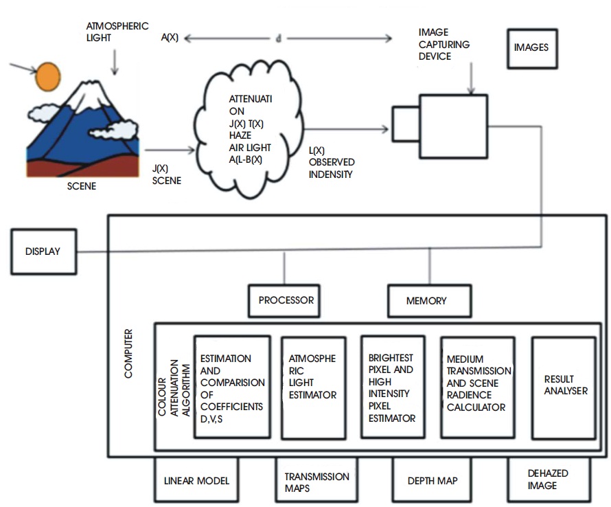
Figure 2. : System Architecture of Proposed System
Narasimhan and Nayar, (2003) and McCartney (1975) have proposed a scattering model to describe the hazy image which can be expressed as,
where I, J, K are 3-dimensional vectors in RGB, x is the position of pixel, β is the scattering coefficient which is considered to be in homogeneous condition, I is the hazy image, J is the scene radiance, A is the atmospheric light, t is the medium transmission which is caluculated using equation (2), if depth is given in ideal case the depth is considered to be in the range 0 to +infinity.
Equation (3) shows the intensity of pixel, where depth tends to infinity, can stand for atmospheric light A. If the value of depth is huge the transmission coefficient will be small, thus a threshold value, d threshold which must be found. This is done by,

For the distant objects the d threshold value will be very large. If all the images are taken too distant then,

Thus A can be calculated by assumption using the equation,
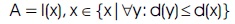
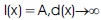
Thus the dehazing was changed into a task of finding depth map. Figures 3 and 4 shows the transmission map and the position of atmospheric light.
Figure 3. Transmission Map
Figure 4. Shows the position of Atmospheric Light
The haze is usually caused by scattering of light that is caused by particles in the atmosphere. Thus the region where the scattering has occurred will have high brightness and low contrast or satuaration. Thus it is concluded that the scene depth changes with density zero haze and difference between brightness and saturation of image is,
Where d is the scene depth, c is the density of haze, v is the brightness of the image, s is the saturation.
The concentration of haze can be found by creating a linear model which is the difference between brightness and saturation pixels. This is done by using the following equation,
Here v is the brightness components or the saturation component, ε(x) the random variable representing the random error of the model, is the position within the image. θ0, θ1 and θ2 are unknown liner coefficients. The coefficient d is the scene depth to be found.
The training sample used here has hazy image and depth map. To learn the coefficients θ0, θ1 and θ2, the training data is important. As there is reliable method to measure depth of outdoor images, depth map is very difficult to obtain. The depth map for each image is found which has same size and from standard uniform distribution the values of pixels are drawn. Then random atmospheric light is generated A (k, k, k) where k is between 0.85 and 1.0. Thus the hazy image is transformed to atmospheric light and depth map.
The depth map can be restored from the depth information d, brightness v, and saturation. Then compare each pixel with the pixels in the neighbourhood. Here, the raw depth map considering the white objects to be distant has been created so, there may be inaccuracy in the dehazed image. Figure 5 shows the depth map that is recovered and smoothened.
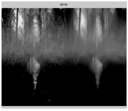
Figure 5. Depth Map Recovered and Smoothened
The scene radiance recovery is done by estimating scene radiance J, by using the coefficient depth d and atmospheric light. The following equation is used for this purpose,

The value of transmission t(x) is considered to be between 0.1 and 0.9, so that only less noise will be produced. Thus the equation used to recover the scene radiance is,

Here, J is the dehazed image which is to be recovered. The coefficient β determines the intensity of transmission map. β used here is considered to be a constant in homogeneous regions. If the value of β is considered very small the image will be hazy in distant regions, but if large value is considered it will be over transmission. Thus is considered to be 1.0, a moderate value.
In this module, the efficiency of proposed dehazing algorithm had been checked. Different images shown in Figures 6-10, and their different values such as Mean Square Error (MSE), Peak Signal to Noise Ratio (PSNR), and normalized cross correlation of image. The MSE or mean square deviation of an estimator measures the average of the squares of the dehazed image and original image and compares them. PSNR is also found to the noise which is in the dehazed and original hazy image. The other method used for finding the errors and efficiency is normalized cross correlation method in which the correlations between both estimator and dehazy image are found by cross checking both images. All these values are found for the comparison of dehazed and hazy image. He et al.'s method has been compared with the proposed method based on real-world images. Compared with the results of the He et al.'s algorithm, the proposed results are free from over satuaration as displayed in the Figure 11, the sky and cloud in the images are clear and the details of the mountains are enhanced moderately.
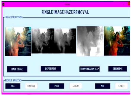
Figure 6. Haze Removal Done with Experimental Result Analysis in MATLAB
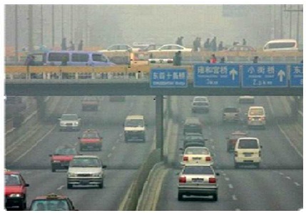
Figure 7. Hazy Image
Figure 8. Depth Maps
Figure 9. Transmission Map
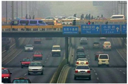
Figure 10. Dehazed Image
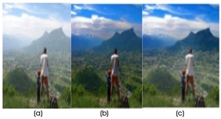
Figure 11. Qualitative Comparisons of He et al.'s and our Methods based on Real-World Images (a) Hazy Image, (b) He et al.'s (2011) Result, (c) Proposed Method Result
In this paper, a method called color attenuation prior algorithm has been proposed, which can do Haze removal of single image very efficiently and easily. It is much better than the old methods used. In this method, the depth map using a linear model has been found and then the transmission map is created with which depth information can be found very easily. But the proposed method has a demerit. The atmospheric coefficient (β) used here has to be considered in homogenous atmospheric condition. For example, a region which is kilometers away from the observer should have a very low value of β. So, this method cannot be used if the atmospheric condition is inhomogeneous. To overcome this challenge, some physical advanced models can be taken into account.
The authors would like to thank all the anonymous reviewers for their valuable comments and suggestions. They would like to thank their tutors for their enthusiastic assistance in improving the clarity of this article.