Artificial Neural Networks (ANNs) are archetypes of the biological neuron system, derived from the capabilities of the human brain. The construction of ANN being derived from the concept of brain functioning, a Neural Network (NN) can be said as hugely replicated network of a huge number of neurons that is processing elements (Dony & Haykin, 1995). ANNs are used to summarize and prototype some of the functional aspects of the human brain system in an effort so as to acquire some of the computational strengths of human brain (Xu, Nandi, & Zhang, 2003). Recently, ANNs are applied in areas in which high rates of computation are essential and deemed as solutions to problems of image compression (Liu, 2007). Generally, two stage approach is put forward for enhancing the performance of compression methods (Patel & Agrawal, 2013). Firstly, a method for compression by using ANN technology has to be developed to improve the design. Secondly, NN has to be applied to develop compression methods (Srivastava & Singh, 2015). Backpropagation algorithm is an extensively used learning algorithm for use in ANNs. With generalization ability and high accuracy, the feedforward neural network architecture is best capable of approximating most problems of compression (Veisi & Jamzad, 2009). This architecture is based on the learning rule of error correction. Error propagation contains two passes through different layers of network. The effect of input vector's application to the sensory nodes of the network transmits through the network layer by layer in the forward pass. In the end, a set of outputs are produced as an actual response of this process (Ahamed & Chandrashekarappa, 2014). All the synaptic weights of the networks are fixed during the forward pass only and adjusted according to the need of error correction during the back pass (Younis & Khalil, 2006). The error signal is produced when the actual output of the network is deducted from the expected output. Through the network, error signal is transmitted backward in contrast to the direction of synaptic situations. Synaptic weights are adjusted, until the real output of the network so produced is closer to the wanted output (Wilamowski, Chen, & Malinowski, 1999). From this knowledge of backpropagation neural networks, image compression and decompression can be achieved.

Image compression reduces the size of data that is needed to construe an image by reducing redundancy in image pixels. The two basic types of image compression are lossless compression and lossy compression. The three basic data redundancies are

1) interpixel 2) psychovisual 3) coding.

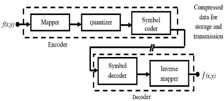
The elimination of one or more of these data redundancies results in image compression. The process of image compression comprises two distinct blocks such as an encoder and a decoder. Figure 1 shows the block diagram of image compression.

Figure 1. Basic Image Compression Block Diagram

An Artificial Neural Network (ANN) is a data processing pattern. ANN is inspired by the architecture of human brain. The original structure of data processing system is the crucial portion of this model (Charif & Salam, 2000). In order to resolve definite problems, huge numbers of exceedingly interconnected data processing elements (neurons) are used. Through a learning progression, an ANN is designed for a precise application such as pattern recognition or data classification. Adjustments to the synaptic connections that exist between the neurons lead to refinement of error in networks. ANN is a structure architected on the model of human brain structure and has many names in the field, for example, neurocomputing. Neural Networks can be used to excerpt patterns and identify trends, which are otherwise not possible to be perceived by computers or humans as they have a particular capacity to produce meaning from complex data. A trained NN can be deemed as “proficient” in the grouping of information, it is used to evaluate. The architecture of the Neural Network is shown in Figure 2.

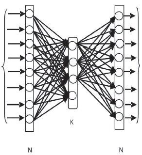
Figure 2. Architecture of Neural Network

Neural Networks being similar to brain are occasionally called machine-learning algorithms due to their acquisition of knowledge from experience. The network learns to solve a problem by modifying its connection weights (training). The strength of nodes between the neurons is assigned as a synaptic weight value for the particular node. The ANN acquires novel information by varying the connection weights of nodes. The learning skill of ANN is influenced by its architecture and the algorithm selected for the purpose of training. The learning method will be one of the three patterns: reinforcement learning, unsupervised learning, and supervised learning. Supervised learning is essentially used for image compression purposes. The block diagram for the training process is shown in Figure 3.

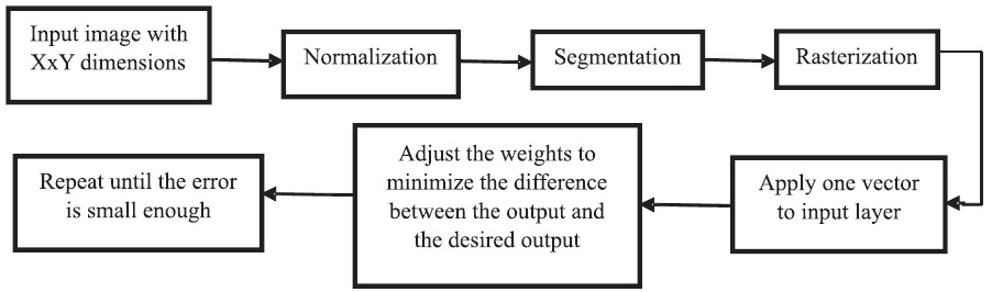
Figure 3. Block Diagram for Training Process

To achieve the object of data compression to the required level, the basic step is to determine the size of the network that is required to perform. Network architecture is to be designated, to offer a sensible image reduction factor. The network is a feed forward network containing three layers, one input layer with N neurons, one output layer with N neurons, and one hidden layer with K neurons. With backpropagation of error measures, the network is trained using a set of patterns to produce the desired outputs same as the inputs. The original image can be reconstructed, by propagating the compressed image to the output units in identical networks, when the values produced by the hidden layer units in the network are read out and transmitted to the receiving station. ANN can be a linear or non-linear network according to the transfer function employed. The most common nonlinear function was sigmoid activation function, which was employed for different Neural Network problems as given in equation (1).

(1)

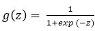
where 'z' is linear sum of input signals after weighing them with the strengths of the respective connections. The output Z_K of the K^th neuron in the hidden layer in  feedforward neural network is given as,

(2)

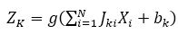
The output Y_N of the N^th neuron in the output layer is given by,

(3)

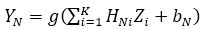
In the above equations, b is the bias, X and Y are input and output layers with N neurons, respectively and Z is the hidden layer with K neurons. J and H represent the weights of compressor and de-compressor, respectively. When the weights converge to their true values, the iterative process of the Neural Network training is stopped. The compression and decompression processes using neural network structure are shown in Figures 4 and 5, respectively. The block diagram for image compression and decompression using backpropagation Neural Networks is shown in Figure 6.

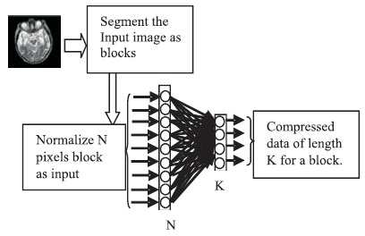
Figure 4. Neural Network Structure for Compression

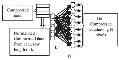
Figure 5. Neural Network Structure for Decompression

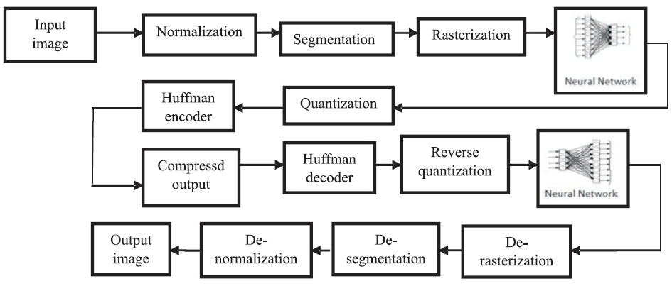
Figure 6. Block Diagram for Image Compression and Decompression using Back Propagation Neural Network

A procedure that modifies weights and biases a network is called training algorithm. Training rule has been applied to train network for image compression. The algorithms of MRI compression at high bit rate are explained in detail in this section.

5.1 Gradient Descent Algorithm

The most widely used training algorithm is multilayer perception (MLP), which is a Gradient Descent (GD) algorithm. It accords the difference ∆W_nk, the weight of a connection between neurons n and k, by equation (4).

(4)

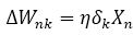
Here η is learning rate parameter

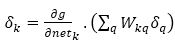
The factor δ_k for output neurons is as,

(5)

Here, net_k is the total weighted sum of input signals to neuron k and Y_n^(t) is the target output for neuron k.

The equation for hidden neurons is as,

(6)

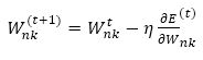
As there are no target outputs for hidden neurons, the difference between the target and actual output is replaced by the weighted sum of the δ_q terms already obtained for neurons (q) connected to the output of k. The method usually adopted to expedite the modification of weights is given as,

(7)

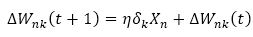
where ∆W_nk (t+1) is weight change in epoch t+1.

5.2 Resilient Backpropagation Algorithm

The conventional backpropagation (BP) learning algorithm uses the partial derivatives of the error function (i.e., the gradient) to minimize the global error of the NN by performing a gradient descent as given in equation (8).

(8)

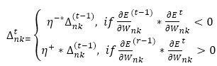
The choice of the learning rate parameter η, which scales the derivative has an important effect on the time needed until convergence. Resilient backpropagation (RP) algorithm is a local adaptive learning method, much faster and stable than other usual variations of the backpropagation algorithms. The elimination of negative and un-expected influence of the size of the partial derivative on the weight step is its basic principle. So, the direction of the weight modification is indicated by only the sign of the derivative. The size of the update is given in equation (9) by a weight specific update value ∆nk and update values are determined from equation (10).

(9)

(10)

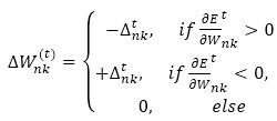
where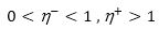

The modified values are determined from the following equation (11).

(11)

The RP learning algorithm is based on learning by epoch; that means after each training, pattern has been obtained and the gradient of the sum of pattern errors is known, and the weight update is performed only after the gradient information is completely available. Some authors have noticed that while using the standard backpropagation method, the weights in the hidden layer are updated with much smaller amounts than the weights in output layer and hence modify much slower. All of the weights growing uniformly is another advantage of RP.

5.3 Levenberg Marquardt Algorithm

The Levenberg Marquardt Algorithm is best adoptable to NN training, where the performance index is the mean squared error. The performance index to be optimized for LM algorithm is defined in equation (12).

(12)

Here, W= [w₁ w₂ w₃…….. w_M]^T consists of all weights of the network, d_kn is the desired value of the k^th output and the n^th pattern, a_kn is the actual value of k^th output and n^th pattern, M is the number of weights, N is the number of patterns, and K is the number of network outputs. Equation (12) can also be expressed as equation (13).

(13)

Here E is the Cumulative Error Vector (for all patterns)

From equation (13), the Jacobin matrix is defined as,

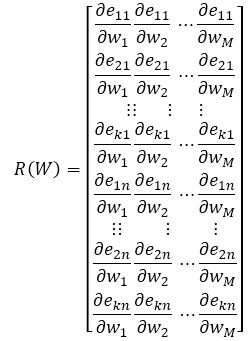
The weights are calculated using equation (14)

(14)

Here “I” is identity unit matrix, “L” is a learning factor, and “R” is Jacobin of k output errors with respect to M weights of the neural network. For L=0, it modifies as the Gauss- Newton method. If “L” is huge, then it modifies as the steepest decent algorithm. To secure convergence, the “L” parameter is automatically adjusted for all iterations. The LM algorithm needs computing Jacobin R matrix at each iteration and the inversion of R^TR square matrix.

Various training algorithms of feed forward backpropagation neural networks are compared using two error metrics. They are the Peak Signal to Noise Ratio (PSNR) and Mean Square Error (MSE). The MSE is the cumulative squared error between the original and the decompressed image and is given in equation (15).

(15)

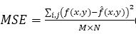
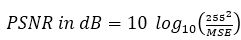
where M x N is the size of the image, M is the number of rows, N is the number of columns, f represents the original image, and ^f represents the decompressed image. The quality of image coding is typically evaluated by the PSNR defined in equation (16) as,

(16)

Compression Ratio (CR) is the ratio of number of input neurons to the number of hidden neurons and is given in equation (17).

(17)

where n_i is the number of input neurons and n_h is the number of output neurons. The three back propagation learning algorithms: GD, RP, and LM have been implemented on four MR brain images, Huntington, Picks, Motor_Neuron, and SubAcute_Stroke. The original brain images of Huntington, Picks, Motor_Neuron, and SubAcute_Stroke are shown in Figure 7. The code has been run for 500 epochs using Matlab R2015a. Tables 1 to 4 give the comparison of the performance metrics of three algorithms for 4×4, 8×8 block sizes with 4 and 9 hidden neurons on test images. These results demonstrated that the average PSNR value obtained by LM algorithm is better and MSE is less when compared to that of RP and GD algorithms. The results of these experiments proved that by using the LM algorithm, the simulation and encoding times are almost similar when compared to that of other algorithms. As it can be seen from the tables, the training time for GD and RP algorithm is almost similar, but it is high for LM algorithm. The change in PSNR values and MSE values with respect to block sizes 4 x 4 and 8 x 8 with 4 and 9 hidden neurons for test images Huntington, Picks, Motor_Neuron, and SubAcute_Stroke have been shown in bar graphs in Figures 12 to 15 (a, b, c and d). From bar graphs, it can be observed that the PSNR values, when image is segmented in 4 x 4 blocks, are greater than the values of PSNR when image is segmented into 8 x 8 blocks for all algorithms. For LM algorithm, as the number of hidden neurons increase, PSNR value increases and MSE value decreases and for RP and GD algorithms, as the number of hidden neurons increases, PSNR value decreases, and MSE value increases. Figures 8 to 11 show the decompressed images of various training algorithms for test images Huntington, Picks, Motor_Neuron, and SubAcute_Stroke before (a, b, and c) and after (d, e, and f) average filter, respectively. Here average filter is used to enhance the quality of decompressed image. From the obtained decompressed images, it is observed that image quality is more for LM algorithm when compared to the other two algorithms. The Neural Network training has been shown in Figure 16 (a, b, and c). The performance plot in the change in MSE has been plotted with respect to 500 epochs is shown in Figure17 (a, b, and c).

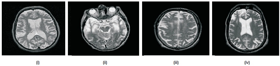
Figure 7. Test Images: (i) Huntington (ii) Picks (iii) Motor_Neuron (iv) SubAcute_Stroke

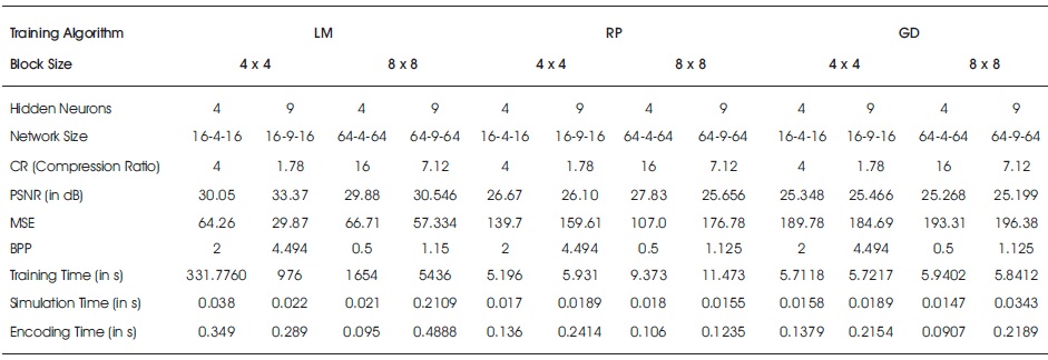
Table 1. Comparison of Performance Metrics of Three Algorithms for Huntington Brain Image

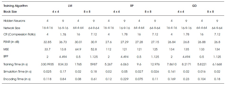
Table 2. Comparison of Performance Metrics of Three Algorithms for Picks Image

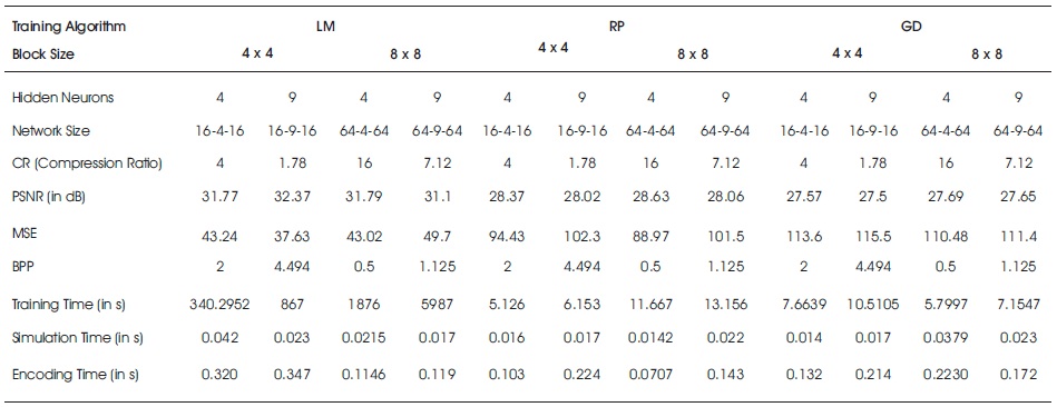
Table 3. Comparison of Performance Metrics of Three Algorithms for Motor_Neuron Brain Image

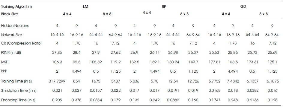
Table 4. Comparison of Performance Metrics of Three Algorithms for SubAcute_Stroke Brain Image

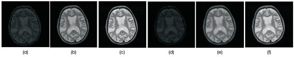
Figure 8. Decompressed Images of various Training Algorithms GD, RP, and LM for Huntington Brain Image for 4 Hidden Neurons with 4 x 4 Block Size before (a, b, c) and after (d, e, f) Filter respectively

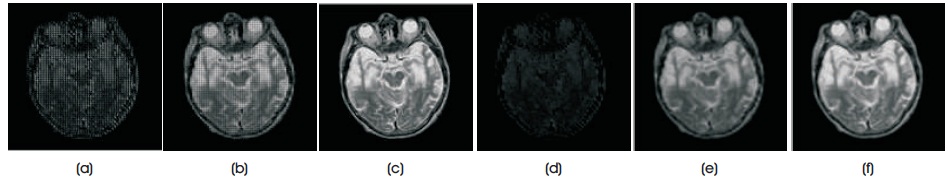
Figure 9. Decompressed Images of various Training Algorithms GD, RP, and LM for Picks Brain Image for 4 Hidden Neurons with 4 x 4 Block Size before (a, b, c) and after (d, e, f) Filter respectively

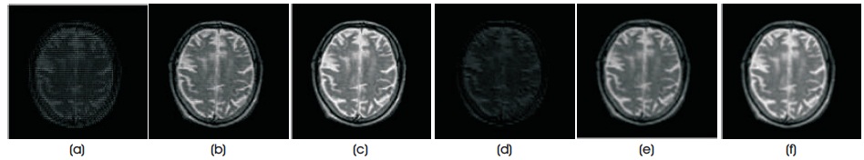
Figure 10. Decompressed Images of various Training Algorithms, GD, RP, and LM for Motor_Neuron Brain Image for 4 Hidden Neurons with 4 x 4 Block Size before (a, b, c) and after (d, e, f) filter, respectively

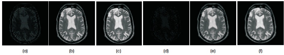
Figure 11. Decompressed Images of various Training Algorithms GD, RP, and LM for SubAcute_Stroke Brain Image for 4 Hidden Neurons with 4 x 4 Block Size before (a, b, c) and after (d, e, f) Filter respectively

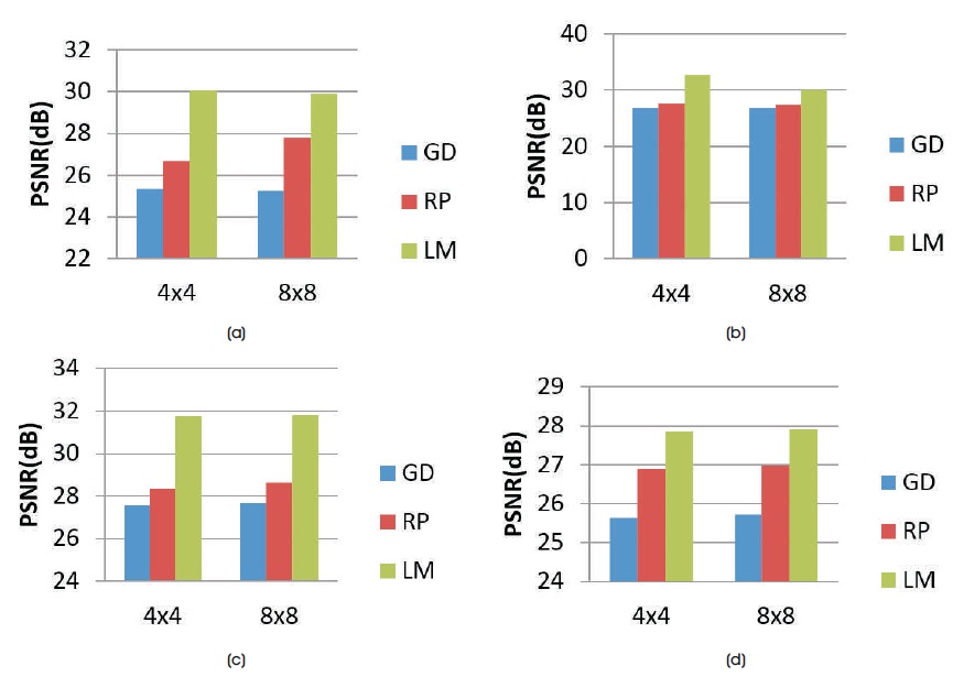
Figure 12. Comparison of the PSNR Values of various Training Algorithms for 4 Hidden Neurons with 4 x 4 and 8 x 8 Block Size of Decompressed Images of Test Images (a) Huntington (b) Picks (c) Motor_Neuron and (d) SubAcute_Stroke

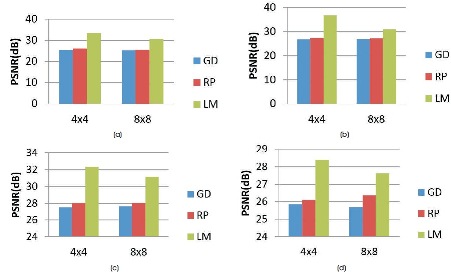
Figure 13. Comparison of the PSNR Values of various Training Algorithms for 9 Hidden Neurons with 4 x 4 and 8 x 8 Block Size of Decompressed Images of Test Images (a) Huntington (b) Picks (c) Motor_Neuron and (d) SubAcute_Stroke

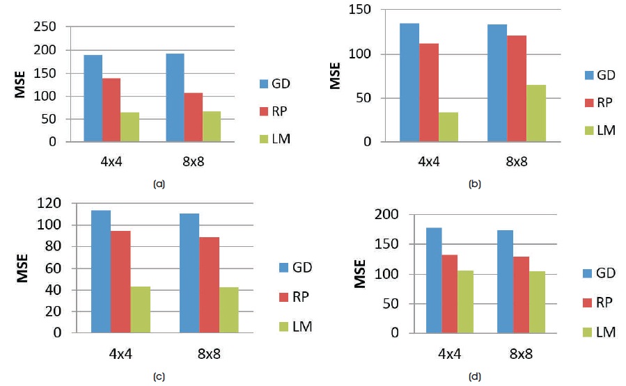
Figure 14. Comparison of the MSE Values of various Training Algorithms for 4 Hidden Neurons with 4 x 4 and 8 x 8 Block Size of Decompressed Images of Test Images (a) Huntington (b) Picks (c) Motor_Neuron and (d) SubAcute_Stroke

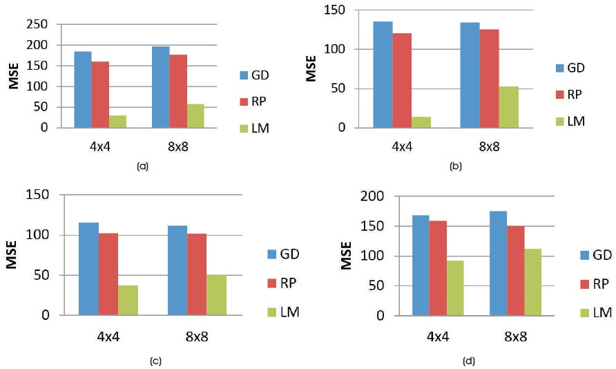
Figure 15. Comparison of the MSE Values of various Training Algorithms for 9 Hidden Neurons with 4 x 4 and 8 x 8 Block Size of Decompressed Images of Test Images (a) Huntington (b) Picks (c) Motor_Neuron and (d) SubAcute_Stroke

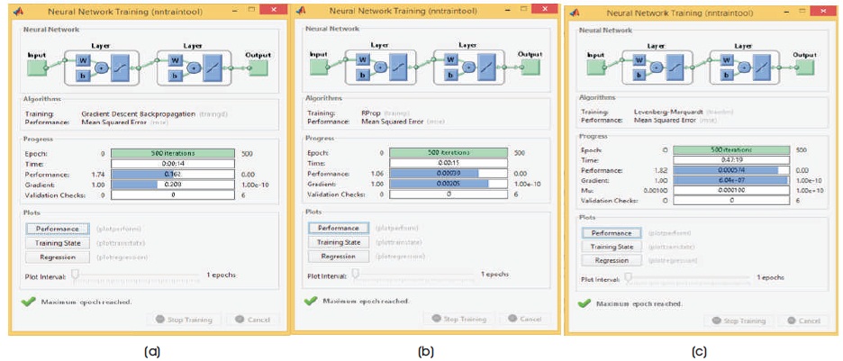
Figure 16. Neural Network Training for Huntington brain Image with 9 Hidden Neurons of 4 x 4 Image Block Size (a) GD (b) RP (c) LM

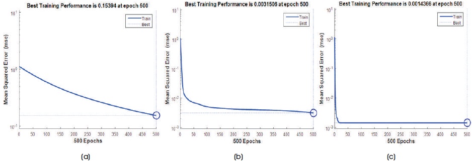
Figure 17. Performance Plot with MSE vs. Epochs for Huntington Brain Image with 9 Hidden Neurons of 4 x 4 Image Block Size (a) GD (b) RP (c) LM

The regression plot is shown in Figure 18 (a, b, and c). From plots, it can be observed that regression plot is more linear for LM algorithm and almost reaches the ideal fitness graph when compared to the other two algorithms. Also in the performance plots, the mean square error is less for LM algorithm.

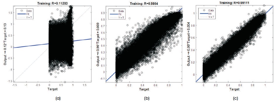
Figure 18. Regression Plot for Huntington brain Image with 9 Hidden Neurons of 4 x 4 Image Block Size (a) GD (b) RP (c) LM

The backpropagation neural networks are used along with quantizer and huffman encoder in image compression system. The network is trained by using three different algorithms: Levenberg Marquardt algorithm, Resilient backpropagation algorithm, and Gradient Decent algorithm. These algorithms are tested on four different MRI brain images of different resolution. The performance metrics, performance plots, training state plots, and regression plots have been compared for all three algorithms. It is found that Levenberg Marquardt algorithm has shown more accurate results with less Mean Square Error and high PSNR when compared to the other two algorithms. The present work can be extended to transformed based vector quantization to the areas in which high rates of computation are essential and deemed as solutions to image compression issues.