[1]
Compressive technique is also known as compressive sampling in signal processing domain and its recent algorithm can be integrated into the MRI reconstruction pipeline for acquiring the complete MR data. The proposed work is based on the recursive iterative adaptive filtering technique based on every injection of random noise in the unobserved portion of the spectrum. The proposed volumetric filter attenuates the noise and relevant features from the incomplete k-space measurements which is required for the clinical practice. The proposed algorithm is based on stochastic approximation method with regularization parameter enabled by a spatial adaptive block-wise volumetric filter. The effectiveness of the proposed reconstruction algorithm is compared with CT reconstruction algorithm radon inversion from sparse projections, spiral, radial, and limited angle tomography. From the reconstruction algorithm it is observed that it achieves exact reconstruction from phantom data even at small projections. The accuracy of this method is to compete with the compressed sensing field. The proposed algorithm is tested on different sampling trajectories, especially on non- Cartesian data and reconstruction of volumetric phantom data with non-zero phase from noisy and incomplete Fourierdomain (k-space) measurements. Experimental results demonstrate that its performance is evaluated by PSNR, SSIM, and execution time.
The most popular algorithm to reconstruct the unknown signal of interest are formulated as convex optimization method which uses mathematical algorithms are consistent with the available data. The optimization is typically constrained by a penalty term expressed as norms which are exploited to enable the sparsity of the assumed image. In MRI, noise or artifact due to the coil sensitivity profile varies due to patient movement and higher magnetic field strength causes, in homogeneity, in the pixel intensity, or bias in the generated complex data. Usually the output of the MRI scanner is a complex raw data with non-zero phase component (Lustig et al., 2008; Wright, 1997; Liang and Lauterbur, 2000; Haacke et al.,1999) (more artifacts in phase domain), generally assuming that the magnitude contains most of structural information (Zhao et al., 2012; Fessler and Noll, 2004; Funai et al., 2008; Zibetti and De Pierro, 2010). In most of the literature only MR magnitude images are considered for post processing applications. In this work, both magnitude and phase are considered and are independently regularized to preserve the edges and features for clinical applications.
The dataset is obtained from a web database The test data of the experiment is Brain-Web phantom and 3-D Shepp-Logan phantom (Vincent, 2006; Schabel, 2006) of size 128×128×128 voxels.
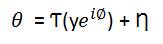
The observation model for the volumetric reconstruction problem is given by,
where θ is the transform-domain representations of the unknown volumetric data having magnitude y and absolute (unwrapped) phase ø. Ƭ is Fourier transform and Ƞ is IID. complex Gaussian noise with zero mean and standard deviation. Let W be the support of the available portion of the spectrum θ. A sampling operator S is defined as the characteristic (indicator) function XΩ, which is 1 over Ω and 0 elsewhere, The spectrum θ can be represented as,
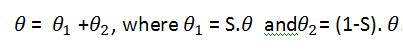
where, θ1 = S.θ and θ2 = (1-S).θ
θ1 and θ2 are the observed (known) and unobserved (unknown) portion of the spectrum, respectively. The goal is to recover an estimate y of the unknown underlying magnitude y from the observed noisy measurements θ1. Since only a small portion of the spectrum is available and since such portion contains noisy measurements, the reconstruction task of the magnitude y is an ill-posed problem.
In this section the reconstruction of volumetric data have been illustrated under the assumption that its phase component is null. The magnitude is equal to the real component and therefore, the reconstruction procedure described in the previous section can be greatly simplified. Since the output of inverse transformation is in general complex due to the noise in the data or numerical errors of the computation, the real component still needs to be extracted after the inverse transformation because the denoising filter is implemented for real inputs. Noise excitation is performed to the unobserved part of the spectrum and then, the (spatial-domain) excited volumetric data is obtained by taking the real part of the inverse transformation of the excited spectrum. Volumetric filtering is accomplished as it was in the above sections, but the application of the VST is no longer needed because the excited spectrum takes the real part and not the modulus. The volumetric reconstruction is eventually produced by the convex combination of denoised data using weights dependent on the excited noise standard deviation.
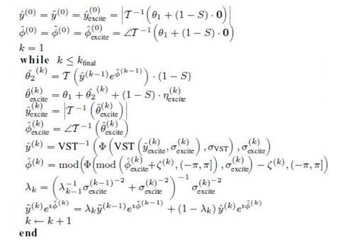
The estimate of the unobserved spectrum is improved by stochastic search driven by the action of adaptive volumetric filter. Further reconstruction is carried out in three cascading stages, namely noise addition, volumetric filtering, and data reconstruction in iterative approach.
The excitation noise is chosen to be complex Gaussian noise with zero mean and variance,
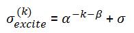
where, α>0 and β>0, are parameters chosen so that the excitation noise lessens as the iterations increase. The variance (exponentially) decreases in order to diminish the aggressiveness of the filtering as the iterations increase. Moreover, the additive term ensures that the excitation noise level converges to the initial noise level in equation (1). The metrics used to measure the performance of the reconstruction are again the PSNR and SSIM. The parameters α and β of the excitation noise are 1.01 and 500, respectively for all measurements.
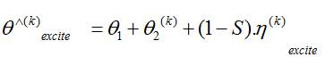
The estimate of the unobserved portion of the spectrum is first extracted using the denoised magnitude and regularized phase produced in the previous iteration. Subsequently, the excited spectrum has been synthetically generate by injecting the unobserved portion of the spectrum with IID. complex Gaussian noise. The volumetric magnitude and phase are obtained by extracting the absolute value (modulus) and angle from the inverse-transformed spectrum, respectively.
The Rician distributed model, need to apply a variance stabilization transform during the filtering of excited magnitude using the standard deviation of the excitation noise. To ensure proper filtering, in particular along phase jumps, we add before denoising and then subtract after denoising a random phase shift. The phase shift is a random variable uniformly distributed between -π and +π defining the phase shift applied to every voxel of excited phase.
The estimates of both magnitude and phase aggregated in a complex recursive convex combination. The iterative procedure can be either stopped after a pre-specified number of iterations or when two magnitude estimates produced at subsequent iterations do not significantly differ from each other. The excited estimate and the aggregated final estimate become equivalent when the system is noise free. But, when the observed spectrum is noisy, the aggregated estimate plays a crucial role in enabling convergence to the expectation of the nonconvergent excited estimate.
The iterative reconstruction algorithm is given as follows.
Design of 3D sampling process involves multi stack of identical 2D slices or trajectories in the MR volumetric data. Reconstruction process involves the measurement of 2D trajectory in the multi-slice stack and is transformed into Fourier k-space domain. Later, the estimated spectrum is observed in 3D transform domain. The sampling trajectories can be classified in to Cartesian and non-Cartesian. The Cartesian data sampling is less susceptible to artifacts and noise and reconstruction process is simple. In case of non-Cartesian trajectory where the data is complex, it requires complicated reconstruction technique, but achieves higher undersampling and faster in acquiring MR data. Today most scanners use non-Cartesian sampling technique for reconstructing the functional MR data and cardiac imaging. For these reasons, the authors use the non- Cartesian trajectories, such as Radial, Spiral, Logarithmic Spiral, Limited Angle, and Spherical and its various parameters are shown in Figures 1 to 4. These trajectories define which K-space coefficients will be retained during acquisition process.
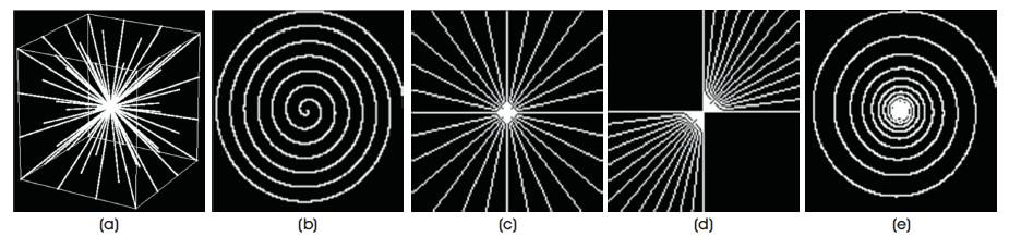
Figure 1. Examples of Different Sampling Trajectories. These Trajectories define which K-Space Coefficients will be Retained during Acquisition Process (a) Radial, (b) Spiral, (c) Logarithmic Spiral, (d) Limited Angle, (e) Spherical
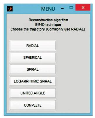
Figure 2. Trajectory Dialogue Box
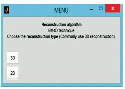
Figure 3. Parameter Profile Dialogue Box
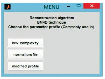
Figure 4. Reconstruction Type Dialogue Box
The performance of the reconstruction algorithm is measured with respect to Peak Signal to Radio Signal (PSNR) and Structural Similarity (SSIM), to test the algorithm over the set of incomplete volumetric data after k final = 1000 iterations, and the experiment is tested over brain web and 3-D Shepp-Logan phantom of size128×128×128 voxels are shown in Figures 5 and 6. The Shepp-Logan is most widely used in medical imaging ( Shepp and Logan, 1974; Gach et al., 2008) and requires the simple reconstruction and the reconstruction task for brain web phantom is performed, which is the most realistic model of MR data used in today's clinical work. Figure 6 shows the PSNR performance versus the number of iterations and it is observed that number of iteration increases, the quality of the image will deteriorate. For better performance the number of iteration is minimum for better noise removal and the computational complexity as shown in Figures 7 to 11.
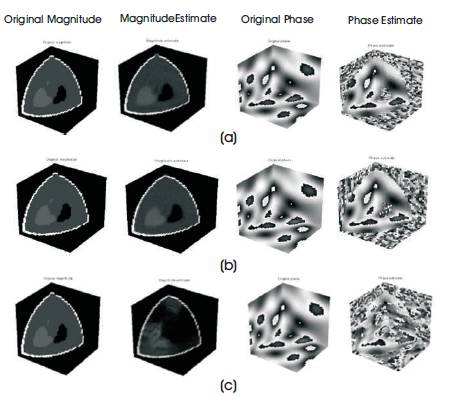
Figure 5. Magnitude and Phase Estimate of Sheep-logan Phantom (a) Radial, (b) Spherical, (c) Spiral
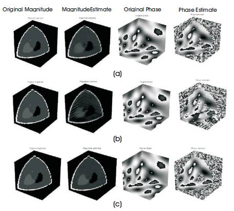
Figure 6. Magnitude and Phase Estimate of Sheep-Logan Phantom (a) Logarithmic Spiral, (b) Limited Angle, (c) Complete
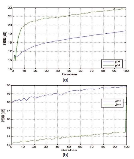
Figure 7. PSNR Values of Estimated Spectrum and Noise Excited Spectrum, and the Change in Values with respect to the Number of Iterations Performed in Case of Radial Trajectory
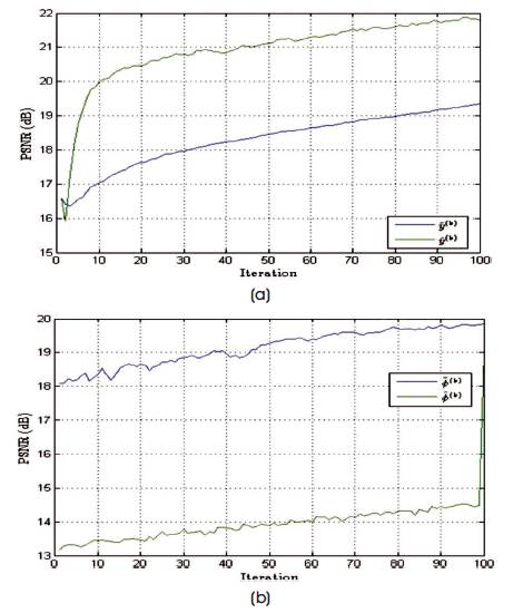
Figure 8. PSNR Values of Estimated Spectrum and Noise Excited Spectrum, and the Change in Values with respect to the Number of Iterations Performed in Case of Spiral Trajectory
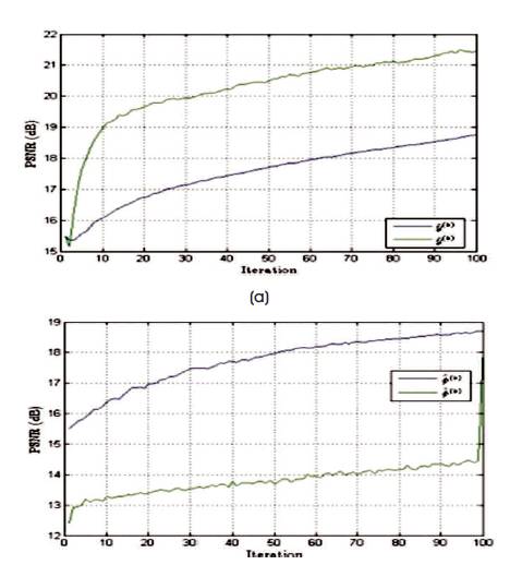
Figure 9. PSNR Values of Estimated Spectrum and Noise Excited Spectrum, and the Change in Values with respect to the Number of Iterations Performed in Case of Logarithmic Spiral Trajectory
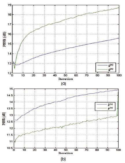
Figure 10. PSNR Values of Estimated Spectrum and Noise Excited Spectrum, and the Change in Values with respect to the Number of Iterations Performed in Case of Limited Angle Trajectory
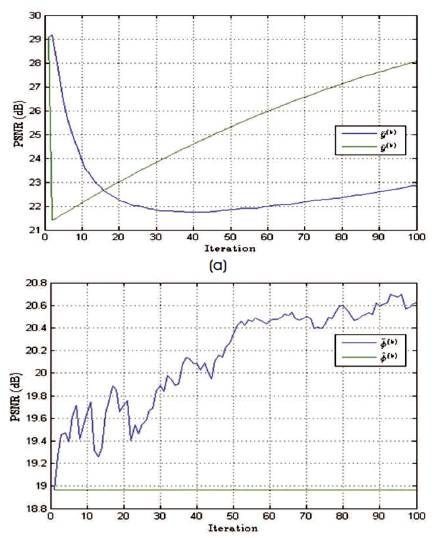
Figure 11. PSNR Values of Estimated Spectrum and Noise Excited Spectrum, and the Change in Values with respect to the Number of Iterations Performed by using the Complete Spectrum for Sampling
The reconstruction performance is noted in Table 1. From the table it is observed that reconstruction performance of the Brain web phantom under the spiral and limited angle shows higher sampling in the noisy case, brain web, and Shepp-Logan phantoms with nonzero phase and its reconstruction performance with non-zero phase are shown in Figure 5 and 6, respectively.

Table 1. PSNR & SSIM for Reconstruction Process after K final Iterations of 1000 of the Brain Web and Shepp-log Phantom of Size 128x128x128 Voxels. Tested are Made both on Noisy and Free Image under Sampling Ratio of 30%
The reconstruction performance of spiral and limited angle shows lower performance than other trajectories, but spherical sampling shows best performance than others which is shown in Figure 5 and 6 and Table 1. The drawback of the spherical sampling is higher scanning time required to complete the acquisition process.
Figure 5 shows the magnitude and phase estimate of Shepp-Logan phantom compared to the original magnitude and original phase of the phantom.
Table 1 gives PSNR and SSIM values (Milanfar, 2013) of running reconstruction program with Brain-Web and Shepp-Logan phantom for sigma values 0% and 5%, respectively. Different PSNR values for different trajectories and computation time for reconstruction of different trajectories and the number of iterations are as shown in Figures 12-14. From these results, it is observed that as the number of iterations increase there is improvement in PSNR, but computation time required is more.
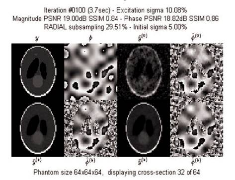
Figure 12. Iteration Window at 100th Iteration
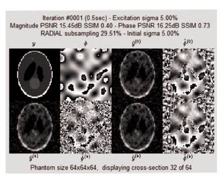
Figure 13. Iteration Window at 1st Iteration
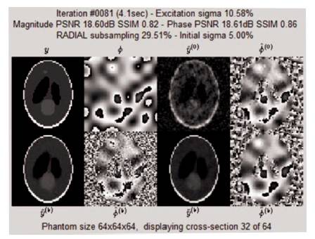
Figure 14. Iteration Window at 81st Iteration
The last magnitude and phase estimates after 100 iterations of reconstruction process of Shepp-Logan phantom with σ = 5% using radial trajectory is shown in Figure 12.
The proposed method uses non-Cartesian sampling trajectories, which allow higher undersampling and fast acquisition times, which mitigate the volumetric reconstruction regularization algorithm. Potential application of non-Cartesian sampling is real-time cardiac imaging that can now be performed by using acquisition times short enough to freeze cardiac and respiratory motion. Myocardial perfusion is another difficult exam that could be improved by non-Cartesian volumetric block wise filtering method.
This research work describes how a non-Cartesian sampling method can be used to reduce MRI data acquisition times. Non-Cartesian sampling of k-space has many advantages, including improved gradient efficiency that allows for faster k-space coverage and the opportunity to collect the center of k-space with every line of data. These non-Cartesian trajectories can be undersampled to further reduce acquisition times and reconstructed with specialized parallel imaging algorithms. The combination of non-Cartesian trajectories and parallel imaging reconstructions allow for larger accelerations and faster scan time than either technique individually, which opens new opportunities for higher spatial and temporal resolutions in many clinical applications which is left for future enhancement.