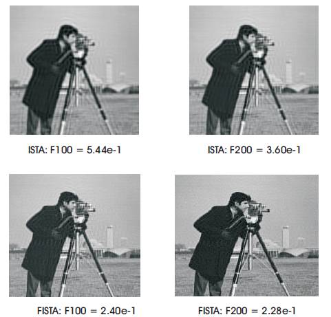
Figure 1. Iterations of ISTA and FISTA methods for deblurring of the cameraman
Image blur is a very difficult problem. Now a days, deblurring plays a vital role in digital image processing. Image deblurring has infinite solutions which are unstable because it is used to make the picture sharp and useful. So, to find the best solution for adjusting the regularization parameter, the number of iterations of the algorithm are used to address the optimization problem. This method well estimates the recovered image, but the residual image is a poorly deblurred image and it exhibits structured artifacts that are not spectrally white. Now in the proposed criterion, the same procedure mentioned above is repeated and the regularization parameter is chosen and the algorithm is decided to stop at the best Signal to Noise Ratio (SNR). Tests will be performed on monochrome and color images with various synthetic and real life degradations to get better results.
Generally images are classified into two types viz., constrained domain and unconstrained domain images. There is no disturbance of light and such images are referred to as constrained domain images, and some images are adjusted before hand to facilitate usage and there can be disturbance of light and posing problems, and these images are referred to as unconstrained domain images. Even by recording the image using camera, the image has more or less blur occuring in every image, due a lot of interference in camera or in the environment. Image deblurring is the general framework used to convert the measurements of the observed image into information about a physical object or system where the observed image is to be made as the convolution of a sharp image by using blur filter with or without noise (white and Gaussian). Wide range of applications in image deblurring are medical imaging, photography, survelliance etc. Mainly Image deblurring is classified into two types, blind and non-blind. If the blurring kernel is to be known, it is referred to as non-blind deblurring; where as if both the image and the blur kernel are unknown, it is referred to as blind de-blurring.Non-blind methods are much narrower than the blind methods. In most cases, the response of an imaging system to a point source is referred to as the point spread function which is not known with good accuracy. So, non-blind methods are very sensitive to mismatches between the PSF (Point Spread Function) used by the method and the true blurring PSF, and a poor knowledge of the blurring PSF normally leads to poor deblurring. In ID problems, the degraded image is designed as y=h*x+n, where 'y' is degraded image,'x' is original image,'n' is noise and h is the point spread function of the blur operator. In BID, to find 'x' and 'h 'from 'y' and in NBID to find 'x 'from 'y 'and 'h' still after many researches have been done, the blur operator in NBID is of ill-conditioned nature. So, there is a slight mismatch between the assumed blur and true one. So we have to overcome this problem by using an image regularizer, or prior the weight of which has to be tuned [1], [2] and the ratio of underlying wavelet/frame-based methods [3], [4]. In BID the blur operator is not of illconditioned nature, but it would still inherently be illposed. Most BID methods limit the class of blur filters, either in a hard way or soft way, using parametric models in hardway [5],[6] and use of priors/regularizers in soft way [7], [8]. It estimates the main features of the image, after using a large regularization weight and gradually knowing the image and filters details by slowly decreasing the regularization parameter. The main drawback is that it requires manual stopping and choosing the final value of the regularization parameter. The difference between the observed image and the blurred estimate equals to that of the noise and this is referred to as discrepancy principle. Two popular criteria generalized cross validation and Lcurve [9] are developed and mainly applied to linear method and also used in non-linear methods. Most existing methods require regularization parameters to be empirically selected. For example, SURE-based approaches assume full information about the degradation model but are not suitable for BID. In the proposed criterion, that can be used to adjust the regularization parameter and stopping iterative ID methods. It is also suitable for both NBID and BID problems. In the observed image, the noise is spectrally white. The ratio is based on measures of spectral whiteness and it represents the fitness of the current estimates to the degradation model.
After many researches have been done, image deblurring is categorized into two types, which are blind and non blind deblurring. To remove the blur from an image, the deconvolution operation is originated. If the blur kernel or PSF is known, it is referred as non-blind deconvolution otherwise, it is referred to as blind deconvolution. So, to discuss the methods of each algorithms, it should be adopted in certain circumstances.
It is also known as the classical linear image restoration problem. Non-blind deblurring is a challenging problem. PSF may vary the true blurring mechanisms which leads to poor deblurring results, and also two difficulties are faced by non-blind deconvolution. The noise is present in the blurred image and ripples around the edges. Even if the noise is very weak, it strongly contaminates the deblurred image. To avoid this difficulty, many non-blind deconvolution methods are used, and the prior information about the image to be recovered are studied.
A recent work manages ISTA (Iterative shrinkagethresholding algorithm) for solving linear inverse problems in image processing. This method converges quite slowly, so as to move the new method FISTA (fast iterative shrinkage-thresholding algorithm) which preserves the calculations that are simple compared with ISTA, but global rate of convergence are significantly better both theoretically and practically. Results for wavelet-based image deblurring exhibit that the capacity of FISTA is faster than ISTA by several orders of magnitude [10]. The function value of ISTA after 1000 iterations, is still worse (that is, larger) than the function value of FISTA after 100 iterations (Figure 1).
Figure 1. Iterations of ISTA and FISTA methods for deblurring of the cameraman
It is referred to as the two-step IST (TwIST) algorithm which exhibits much faster convergence rate than IST for illconditioned problems. The main aim of this method is to keep the good denoising performance of the IST scheme and to be able to handle ill-posed problems efficiently. Figure 2 shows TV-based image restoration from 40% missing samples observed image and restored image.
TwIST is to be converged much faster than the original IST in severely ill-conditioned problem to speed up and reach the two orders of magnitude in a typical deblurring problem. Problem of image restoration from missing samples is solved by new method MTWIST [11].
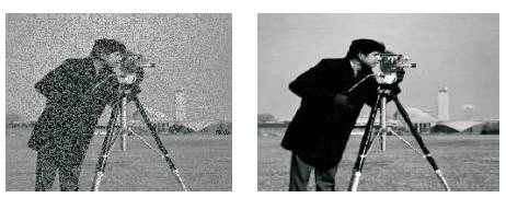
Figure 2. TV-based image restoration from 40% missing samples observed image and restored image
The EM algorithm combines the efficient image representation that can be offered by the Discrete Wavelet Transform (DWT) and diagonalization of the convolution operator obtained in the Fourier domain. It is a general-purpose approach to wavelet-based image restoration with computational complexity compared to that of standard wavelet denoising schemes. The algorithm is arranged between an E-step based on fast Fourier transform (FFT) and a DWT-based on M-step. So the result in an efficient iterative process requires Q (NlogN) operations per iteration. The behavior of the algorithm is investigated and shown under mild conditions. The algorithm converges to a globally optimal restoration. Some features of this method are,
Basic property of an EM algorithm is that it generates a sequence of nondecreasing likelihood values. EM iterations produced a sequence of images and each one has a penalized likelihood value greater than or equal to the preceding image. But several questions remain.
1) Does penalized likelihood values converge to the maximum penalized likelihood?
2) Does the corresponding sequence of images converge to the fixed image and is this limit unique? First is to consider the conditions of the EM algorithm, where it converges to a stationary point of the penalized likelihood function. Second, is to investigate the measure of the curvature of the penalized negative log-likelihood function (Figures 3, 4 and 5).
It leads to a simple procedure that alternates between Fourier domain filtering and wavelet domain denoising [12].Figure 7 shows the deblurring effect.
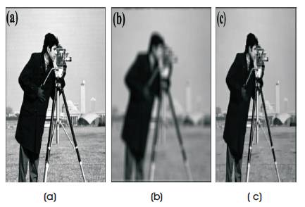
Figure 3. (a) Original image, (b) blurred image, and ( c) restored image using the UDWT version
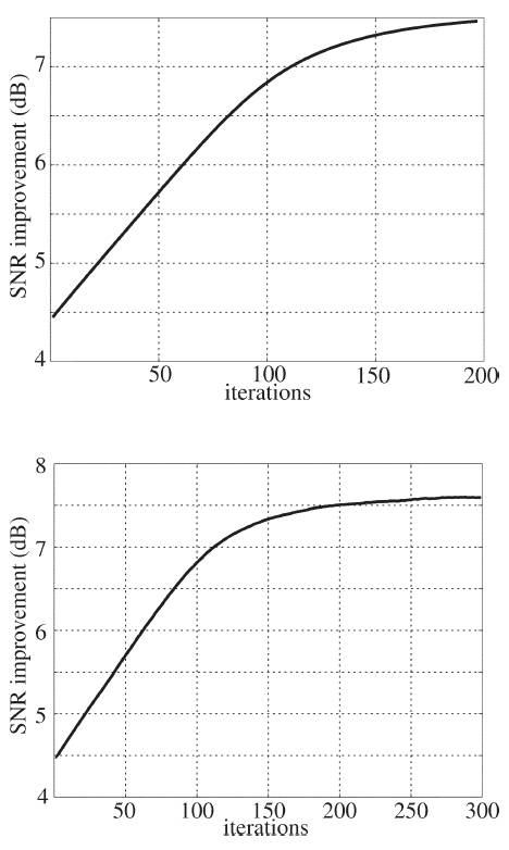
Figure 4. SNR improvement along the iterations of the (top) UDWT-based method and the random shifts method
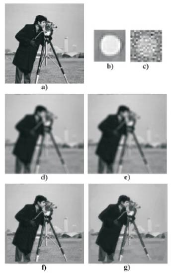
Figure 5. Results of synthetic experiments. a) Original image. b) and c) Filter estimates. Next rows: Left, without noise; Right, with noise. Second row: Blurred images. Third row: Deblurred images
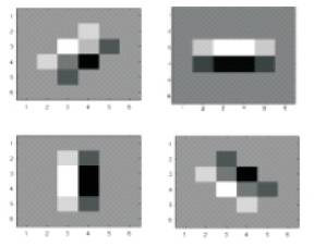
Figure 6. The figure shows the 4 orientations of the edge detection filter. The filter kernels are interpolated for all orientations
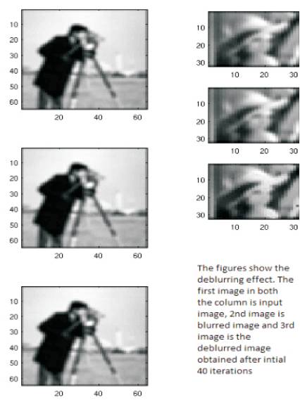
Figure 7. Deblurring effect
After many researches the result at the various intersections have been studied extensively. Previous methods in blind deblurring are very limited. They should not use the generic PSF. Most of them are based on a small number of parameters. Even a slight mismatch between the deblurring PSF and the blurring PSF strongly degrades the quality of the deblurred image. BID suffers from lack of understanding of data.
Very few assumptions are made on blurring filter and original image. Estimation of both deblurred image and blurring filter is made in a progressive way, first taking into account, the main features of the image and then proceeding to smaller details. The results are obtained with synthetically blurred images which are good even when the blur operator is ill-conditioned and the blurred image is noisy. This method yields improvements in real life photographs with focus and motion blurs [13].
1.2.2 Blind and Semi-Blind De-blurring of Natural Images The algorithm works on natural images to different kinds of blurring, and de- blurs the image. In blind approach, that minimal information about the blurring filter is needed to de-blur the image. This method applies to unconstrained blurs and can apply for both gray scale and color images. The algorithm uses the new image prior and increase the Signal to Noise ratio compared to the state of the art approaches [14].
Figure 6 shows the 4 orientations of the edge detection filter. The filter kernels are interpolated for all orientations.
From the above analysis, it can be concluded that it is accurate but not active to different types of blurs and lighting problems to make the deblurring, as it is difficult. In the previous methods, the regularization parameters can be used to stop iterative blind and non-blind deconvolution algorithm. But proposed technique is based on whiteness of the residual image. The proposed method is to be handled for both constrained and unconstrained domain images. It makes weak assumptions about the blurring filter and focus on the main edges of the image and gradually takes details into account. It works on single-frame scenarios, both monochrome and color images and then synthetic and real-life degradations.