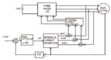
Figure 1. BLDC Motor Drive Control Scheme
The position of Brushless Direct Current (BLDC) rotor is determined by measuring the changes in the Back-EMF. Sensorless control method reduces the cost of the motor as it does not need sensors. This paper presents Bio-inspired optimization technique (Particle Swarm Optimization algorithm) and classical methods of tuning PID control parameters for the automatic speed tracking of BLDC motor. The BLDC is modelled in Simulink in Matlab and Back-EMF waveforms are modelled as a function of rotor position. The proposed methods are effective in reducing the steady state error, rise time, settling time, and peak overshoot. The classical methods such as Ziegler-Nichols (Z-N), Tyreus-Luyben (T-L) methods, and Particle Swarm Optimization (PSO) techniques based on effective objective function Integral Absolute Error (IAE) are proposed for the optimal tuning of PID controller parameters. The results obtained from Particle Swarm Optimization technique are compared with the classical methods.
The BLDC motor came into existence in 1960s. This motor has several advantages such as high efficiency, flat speedtorque characteristics, high speed range, when compared against Brushed DC motor. BLDC motors are electronically commutative motors in contrast to the mechanically commutated brushed DC motor [1]. The position of the rotor can be determined by two methods; one is by using hall effect sensors [6], and the other is by measuring the changes in the back emf in each of the armature coils as the motor rotates which is a sensorless control method [3], [5], [7]. Here the position of the rotor is determined by measuring the changes in the back emf. There were many techniques for the tuning of PID controllers, but each method has one or more difficulties. This paper presents Ziegler-Nichols (Z-N), Tyerus–Luyben (T-L), and Particle Swarm Optimization (PSO) algorithm for tuning PID controller parameters. Particle swarm optimization algorithm solves many optimization problems. This algorithm is based on the social behaviour of bird flocking.
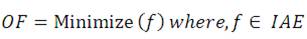
The main objective in the optimal PID-design is to minimize the overshoots and settling time in system oscillations with minimum error. In this paper, two classical methods of tuning and Particle Swarm Optimization algorithm have been used for optimization of PID-parameters. Just like any optimization problem, an objective function needs to be formulated for optimal PID-design.
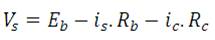
A brushless DC motor is a DC motor turned inside out so that the field is on the rotor and armature is on the stator, having the armature on stator makes it easy to conduct heat away from winding, this is another advantage with brushless motor. The BLDC is supplied from a battery through an inverter. BLDC motor accomplishes electronic commutation using rotor position feedback to determine the current switching [2]. The stator winding work in conjunction with permanent magnets on the rotor to generate a nearly uniform flux density in the airgap. This permit the stator coils to be driven by a constant voltage (hence the name brushless DC), which simply switches from one stator coil to the next to generate AC voltage waveform with a trapezoidal shape [3]. The schematic diagram of BLDC motor drive control is shown in Figure 1.
Figure 1. BLDC Motor Drive Control Scheme
The equations that describe the model is as follows:
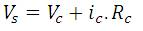
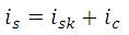
where,
Eb and Rb – voltage and resistance of source, respectively,
Rc - resistance in capacitor, vc - voltage across capacitor,
is - source circuit current, ic - current through capacitor,
is - converter input current.
Voltage equations at the motor side are:
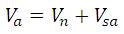
where Vsa , Vsb , Vsc are the inverter output voltages that supply the 3-Ф winding. Va , Vb , Vc are the voltages across the motor armature winding. Vn – voltage at the neutral point.
The stator winding voltages in terms of the winding parameters are expressed as,
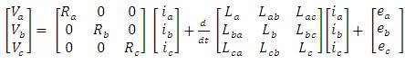
and the electromotive forces of three- phase windings are:
where,
The Torque balance equation of drive system is expressed as,
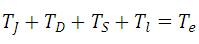
Torque due to Inertia,

where, J – Moment of inertia,
Torque due to viscous friction, TD = B.ωr
where, B – Friction coefficient,
The Electromagnetic torque of 3-phase motor is

The Proportional Integral Derivative (PID) controller operates the majority of the control systems in the world. It has been reported that more than 95% of the controllers in the industrial process control applications are of PID type as no other controller match the simplicity, clear functionality, applicability and ease of use offered by the PID controller [9]. In a PID controller, the proportional, integral and derivative modes has to be tuned, all the three gains combine together for the control of the drive system [10], [13]. The control system becomes unstable if the parameters are not tuned properly, PID controllers provide robust and reliable performance for most systems [4], [16]. The block diagram of PID controller with proposed tuning methods is shown in Figure 2. The main aim of tuning the controller parameters is to reduce rise time, settling time with zero overshoot and without steady state error, for this to happen the classical tuning methods such as Ziegler- Nichols, Tyerus-Luyben, and bio-inspired optimization technique-Particle Swarm Optimization algorithm are proposed.
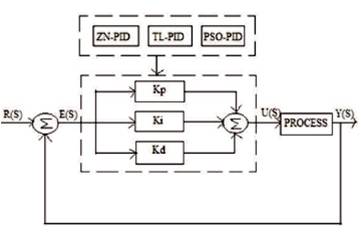
Figure 2. Optimal PID Controller
The Ziegler–Nichols tuning method was developed by John G. Ziegler and Nathaniel B. Nichols. This method that is probably the most known and the most widely used methods for tuning of PID controllers is also known as online or continuous cycling or ultimate gain tuning method. Z–N tuning creates “quarter wave decay”. This is an acceptable result for some purposes, but not optimal for all applications. The Ziegler-Nichols tuning rule is meant to give PID loops best disturbance rejection. Z–N yields an aggressive gain and overshoot – some applications wish to instead minimize or eliminate overshoot, and for these Z–N is inappropriate. The step response of closed loop system with ZN-PID and without ZN-PID is shown in Figure 3, the electromagnetic torque is shown in Figure 4, the back-EMF with ZN-PID is shown in Figure 5, and Three-phase current is shown in Figure 6.
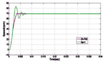
Figure 3. Step Response of Closed Loop System with ZN-PID and without ZN-PID
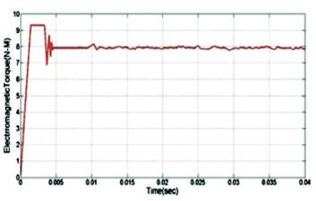
Figure 4. Electromagnetic Torque with ZN-PID
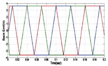
Figure 5. Back-EMF with ZN-PID
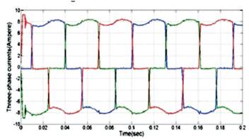
Figure 6. Three-phase Currents with ZN-PID
Step 1: Deactivate integral and derivative control, i.e. set τi =0, τd =0.
Step 2: Start raising the gain kc until the process starts to oscillate. The gain where this occurs is ku and the period of the oscillation is τu.
Step 3: Record the values as ultimate gain (ku ) and ultimate period (τu ).
Step 4: Evaluate control parameters as prescribed by Ziegler and Nichols.
The step response of closed loop system with ZN-PID and with Kp =1 is shown in Figure 3.
The Tyreus-Luyben tuning method developed by Tyreus and Luyben (1997) is based on oscillations as in the Ziegler- Nichols method, but with modified formulas for the controller parameters to obtain better stability in the control loop compared with the Ziegler-Nichols method. The Tyreus-Luyben procedure is quite similar to the Ziegler–Nichols method, but the final controller settings are different. Also, this method only proposes settings for PID controllers. The step response of the system TL-PID and with Kp =1 is shown in Figure 7, electromagnetic torque is shown in Figure 8, Back-EMF waveform with TL-PID is shown in Figure 9, and three-phase currents are shown in Figure 10.
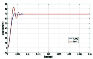
Figure 7. Step Response of Closed Loop System with TL-PID and without TL-PID
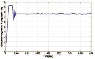
Figure 8. Electromagnetic Torque with TL-PID
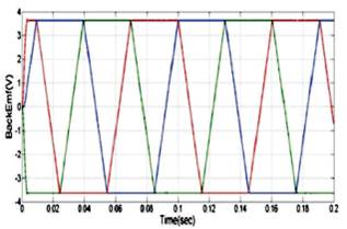
Figure 9. Back-EMF with TL-PID
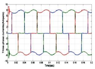
Figure 10. Three-phase Currents with TL-PID
Particle Swarm Optimization (PSO) algorithm is a population based stochastic optimization technique developed by Kennedy and Eberhart in 1995 inspired by the social behaviour of bird flocking or fish schooling [11]. PSO requires only primitive mathematical operators and is computationally inexpensive in terms of both memory requirements and time. A swarm in PSO consists of a number of particles. Each particle represents a potential solution to the optimization task. Each particle represents a candidate solution. Each particle moves to a new position according to the new velocity, which includes its previous velocity and the moving vectors according to the past best solution and global best solution [12]-[15]. The best solution is then kept; each particle accelerates in the directions of not only the local best solution, but also the global best position. If a particle discovers a new probable solution, other particles will move closer to it in order to explore the region. The optimization technique is applied on to the objective functions, which one is most efficient to calculate the individual particle's fitness value. A fairly useful performance index is the Integral of Absolute Error (IAE), and it is expressed in the equation as,
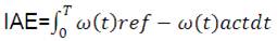
where ω(t)ref is reference speed and ω(t) act is actual speed. IAE integrates the absolute error over time. It doesn't add weight to any of the errors in a systems response. It tends to produce results in a fairly good under damped system. Therefore, the design problem can be formulated as the optimization problem and the objective function is expressed as,
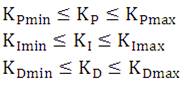
Subjected to constraints,
Step 1: Read the data and generate the initial solution randomly.
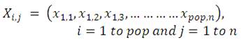
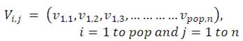
where, pop is population size and n is dimension of the problem.
Step 2: Calculation of fitness value of the objective function using Equation (12).
Step 3: Calculate pbest, i.e., objective function value of each particle in the population of the current iteration is compared with its previous iteration and the position of the particle having a lower objective function value as pbest for the current iteration is recorded.
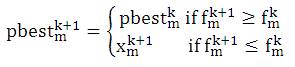
where, k is the number of iterations, and f is objective function evaluated for the particle.
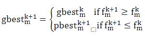
Step 4: Calculation of gbest, i.e., the best objective function associated with the pbest among all particles in the current iteration is compared with that in the previous iteration and the lower value is selected as the current overall gbest.
Step 5: Velocity updating, after calculation of the pbest and gbest, the velocity of particles for the next iteration should be modified by using equation:
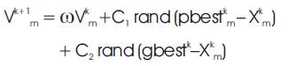
where, the parameters of the above equation should be determined in advance and ω is the inertia weight factor, defined as follows:
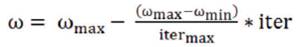
C1 , C2 are the acceleration coefficients usually in range [1, 2 ]. A large inertia weight (w) facilitates a global search while a small inertia weight facilitates a local search.
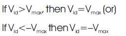
Step 6: Check the velocity components constraints occurring in the limits from the following conditions,
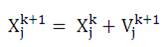
Step 7: Position updating, the position of each particle at the next iteration (k+1) is modified as follows:
Step 8: If the number of iterations reaches the maximum then go to step 9 for gbest otherwise, go to step 2.
Step 9: The individual that generates the latest gbest is the optimal PID parameters at minimum objective function.
The step response of the closed loop system with Particle Swarm Optimization tuning of PID controller and without tuning with Kp =1 is shown in Figure 12. The electromagnetic p torque curve with PSO tuning of PID controller is smoother than the curves with classical methods of tuning as shown in Figure 13. Back-EMF waveforms with PSO-PID is shown in Figure 14, and three-phase current waveforms which are smoother curves than classical tuned methods are shown in Figure 15. The flowchart for the Particle Swarm Optimization technique for the tuning of PID control parameters is shown in Figure 11.
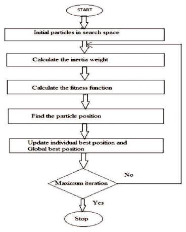
Figure 11. Flowchart for Particle Swarm Optimization
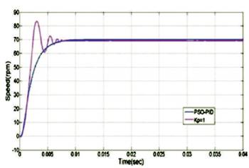
Figure 12. Step Response of Closed Loop System with PSO-PID and without PSO-PID
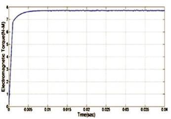
Figure 13. Electromagnetic Torque with PSO-PID
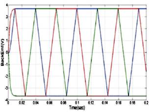
Figure 14. Back-EMF with PSO-PID
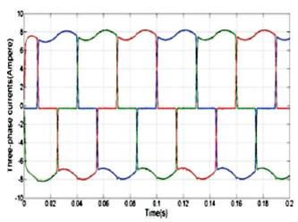
Figure 15. Three-phase Currents with PSO-PID
The electromagnetic torques of ZN-PID,TL-PID, and Particle Swarm Optimization Algorithm shown in Figures 4, 8, and 13 respectively, are compared as in Figure 16 and also comparison of step responses of all three tuning methods is is shown in Figure 17 and have been discussed in this section. The electromagnetic torque curve of PSO-PID is a smooth curve without any fluctuations compared to ZN-PID and TL-PID.
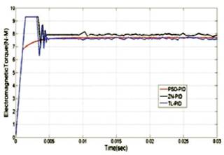
Figure 16. Comparison of Electromagnetic Torques with Proposed Tuning Methods
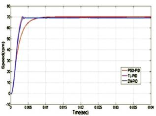
Figure 17. Comparison of Step Responses of Proposed Tuning Methods
In Figure 17, speed responses have been compared. The steady state error (ess ) of PSO-PID is 0.03 rpm, whereas in ZN- PID, it is 0.85 rpm and 0.81rpm in TL-PID. PSO-PID is showing very less steady state error (ess ). The peak overshoot is zero in PSO-PID and ZN-PID, whereas in TL-PID it is 0.29. The peak time of PSO-PID is 0.0131 seconds, which is more than the peak time (tp ) of ZN-PID and TL-PID. The rise time (tr ) of PSO-PID is 0.0091 seconds and for the ZN-PID it is 0.0035 seconds and 0.0032 seconds for TL-PID. The settling time (ts ) of PSO- PID is 0.0133 seconds, ZN-PID and TL-PID is taking less time to settle, but with much steady state error than PSO-PID. The gain values with Particle Swarm Optimization algorithm are Kp =.3484, Ki=4.883, and Kd =0.002.
The controller gain values, peak time (tp ), rise time (tr ), settling time (ts ), delay time (td ), maximum peak overshoot (Mp ), and steady state error (ess ) values obtained from classical methods and Particle Swarm Optimization algorithm are presented in Table 1.
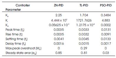
Table 1. Performance Parameters of ZN-PID, TL-PID, PSO-PID
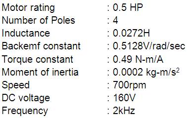
The motor drive used for simulation process has the following specifications:
In this work, the comparison study of classical methods and optimization technique for the tuning of PID control parameters for automatic speed tracking of BLDC motor is obtained through simulation in Simulink in Matlab. The speed-time curve of Particle Swarm Optimization tuned PID controller is smooth without fluctuation, no peak overshoot, and the steady state error are reduced compared to speed-time curves of ZN tuned and TL tuned PID controller, since Particle Swarm Optimization gives better optimal gains of PID controller than the classical Ziegler-Nichols and Tyreus-Luyben methods of tuning PID controller.