
Figure 1. AVR Model
This paper presents three types of optimization techniques; Teaching Learned Based Optimization (TLBO), Harmony Search Algorithm (HSA), and Local Unimodal Sampling (LUS) which are used to tune the controller parameters in Automatic Voltage Regulator (AVR) system. AVR system is used to adjust the terminal voltage of synchronous generator. This paper presents two types of controllers: Proportional-Integral- Derivative (PID) and Proportional-Integral-Derivative- Acceleration (PIDA). Each controller is used with TLBO, HSA, and LUS. For PID controller, these techniques show better performance than Many Optimizing Liaisons (MOL), Gravitational Search Algorithm (GSA), Artificial Bee Colony (ABC), Particle Swarm Optimization (PSO), and Differential Evolution (DE) in previous works. For PIDA controller, these techniques show better performance than Bat Search (BAT), Current Search (CS), Tabu Search (TS), and Genetic Algorithm (GA) in previous works. By comparing both controllers, PIDA shows better response in overshoot and steady state error than PID.
The Automatic Voltage Regulator (AVR) is a device that adjusts or regulates the output voltage within the nominal voltage of synchronous generator under different loading conditions. It controls the value of excitation current in the exciter (which controls magnetic field and induced EMF) to keep terminal voltage at nominal voltage [1]. The output voltage shows instability and slow response due to high alternator field windings inductance and load variation. A controller is used to get better stability and better response by minimizing the Maximum percentage overshoot (Mp ), Rise Time (Tr ), Settling Time (Ts ) and Steady State Error (Ess ).
There are different types of controllers such as: Proportional- Integral-Derivative (PID) [2], Fraction Orders PID (FOPID) [3], Sugeno Fuzzy Logic (SFL) [4,5], Proportional- Integral- Derivative-Acceleration (PIDA) [6], Fuzzy P and Fuzzy I and Fuzzy D [7] and others. Optimization techniques are used to tune the controller parameters due to high order, time delays, nonlinear loads, variable operating points, and others. They are also used to have better transient response, root locus, bode and statistically Receiver Operating Characteristic (ROC) analyses. There are many types of optimization techniques used in tuning controllers of AVR such as Genetic Algorithm (GA) [8], Current Search (CS) [9], Particle Swarm Optimization (PSO) [10,11], Tabu Search (TS) [12], Bat Search (BAT) [13], Taguchi Combined Genetic Algorithm (TCGA) [14], Ant Colony Optimization (ACO) [15], Gravitational Search Algorithm (GSA) [16], Artificial Bee Colony (ABC) [17], Many Optimizing Liaisons (MOL) [18], Local Unimodal Sampling (LUS) [19], Harmony Search Algorithm (HSA) [20, 21] and Teaching Learned Based Optimization (TLBO) [22, 23].
In 2004, Z.L. Gaing performed Particle Swarm Optimization (PSO) with PID controller in AVR system. PSO was compared with Genetic Algorithm (GA) to get better performance in output voltage of the AVR system [24]. In 2007, Mukherjee and Ghoshal performed Craziness based on Particle Swarm Optimization (CRPSO) using Sugeno Fuzzy PID Controller in AVR. CRPSO was compared with GA to get better performance and more robust than GA. This paper shows also that CRPSO is better in performance than PSOPID controller and Hybrid Taguchi Particle Swarm Optimization [25]. In 2008, Anant and Padej wrote a paper using TS in AVR system with PID controller that it has better performance than Ziegler and Nichols method. IAE, ISE, and ITAE are used as objective functions [26]. In 2009, A. Chatterjee, V. Mukherjee, and S.P. Ghoshal used VRPSO and CRPSO to tune Sugeno fuzzy PID controller in AVR system. These techniques showed better performance and response than PSO and GA. This paper showed also that VRPSO performs better than CRPSO [27]. In 2011, Gozde and Cengiz published a paper that showed better performance and tuning, capacity of the Artificial Bee Colony (ABC) optimization than PSO and Differential Evolution (DE) algorithm using PID Controller in AVR system [28]. In 2012, Panda, Sahu and Mohanty prepared the design of PID Controller in AVR using simplified Particle Swarm Optimization which is also called Many Optimizing Liaisons (MOL) algorithm. This paper compared between MOL, ABC, PSO, and DE algorithm and showed that MOL has the best performance on AVR system [29]. In 2012, Deacha calculated and showed that CS using PIDA controller in the AVR system has better performance and response than Genetic Algorithm (GA) and Tabu Search (TS) [30]. Duman, Yorukeren, and Altas concluded that GSA using PID Controller in AVR system has better performance, lower maximum overshoot, lower settling time and rise time than ABC, PSO, and DE algorithm. ITAE is used as objective function [31]. In 2016, Sambariya and Paliwal designed an AVR model using PIDA controller, which is optimized by BAT algorithm. This optimization was compared with Genetic Algorithm (GA), Tabu Search (TS), and Current Search (CS) using PIDA controller. BAT has better performance in output voltage using the three objective functions Integrated Square Error (ISE), Integrated Absolute Error (IAE), and Integral Time-Weighted-Absolute Error (ITAE) [32] .
The rest of the paper is arranged as follows: Section 1 describes AVR system model. Section 2 shows the controllers used (PID and PIDA). Section 3 shows the optimization techniques used (LUS, HSA, and TLBO). Section 4 illustrates different types of objective functions. Section 5 deals with results and comparison between the three optimization techniques in each controller and other techniques. Section 6 is the conclusion of the paper.
An AVR system comprises four main components: Amplifier, Exciter, Generator, and Sensor. These components will be linearized (ignore saturation and non-linearity) using four transfer functions for mathematical modeling as shown in Figure 1. The generator terminal voltage ( ΔVt ) is sensed by a sensor. The signal of the sensor is rectified, smoothed ( ΔVs ), and compared to the input or reference signal (ΔVref ) by the comparator. The output signal of this comparator is the error voltage ( ΔVe ), which is then amplified and sent to the exciter to adjust the excitation current which controls the terminal voltage of generator ( ΔVt ) [1], [24].
Figure 1. AVR Model
Its transfer function is as follows:

where KA : Amplifier gain that ranges from 10 to 40,
TA : Amplifier time constant that ranges from 0.02 to 0.1 A seconds.
Its transfer function is as follows:

where KE : Exciter gain that ranges from 1 to 10,
TE : Exciter time constant that ranges from 0.4 to 1 second.
Its transfer function is as follows:

where KG : Generator gain that ranges from 0.7 to 1.
TG : Generator time constant that ranges from 1 to 2 seconds.
Its transfer function is as follows:

where KS : Sensor gain that ranges from 0.7 to 1.
TS : Sensor time constant that ranges from 0.001 to 0.06 S seconds.
The transfer function will be simplified in the equation below:

Controllers are used to improve stability and dynamic response by minimizing maximum overshoot, reducing settling time, reducing rise time, and improving steady state error. PID controller [2] and PIDA controller [6] are used.
Proportional-Integral-Derivative (PID) controller is simple and robust so it has been widely used in industries. PID controller has burdened problems such as non-linearity, high order, and time delay.
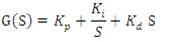
It has three gains: proportional gain (Kp), integral gain (Ki), and derivative gain (Kd) as shown in equation (6) in Laplace d function.
Proportional gain reduces the rise time. Integral gain improves steady-state error. Derivative gain reduces overshoot and improves stability margin.
Figure 2 shows AVR system using PID controller.

Figure 2. AVR System with PID Controller
Proportional-Integral-Derivative-Acceleration (PIDA) controller is expressed in transfer function as in equation (7).

where, Kp : Proportional gain, Ki: Integral gain, Kd : Derivative gain, Ka : Acceleration gain, and “d and e”: filter elements.
PIDA controller is also expressed in polynomial form with parameters Kp , Ki, Kd , Ka , α and β as in equation (8). Figure 3 shows AVR system model with PIDA controller.
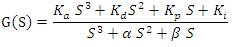

Figure 3. AVR System with PIDA Controller
There are different types of optimization techniques such as: GA, PSO, TLBO, LUS, HSA, CS, TS, BAT, and others used in literature. Figure 4 shows AVR system model using optimization technique which tunes the controller parameters.

Figure 4. AVR System using Optimization Technique for Controller Tuning
The used optimization techniques in this paper are:
This optimization technique takes the best fitness position from random position particle which decreases its sampling range with the new position of the particle using iteration method. This optimization technique overcomes the problem of using a fixed sampling range as it is used in Simulated Annealing (SA) and Hill Climber (HC) algorithm [19].
Steps in LUS algorithm are as follows:
1. Randomly initialize current position  which is found in search space, where
  and n: is dimension of search space.
2. Initialize search range  , where d: is range in search space, Bup is the upper boundary, and Bdown is the lower boundary.
3. Randomly select a vector  where (-D, D) is the initial sample range.
4. It is moved to new position  .
.
5. If  , update the position
  .
.
6. If  , put new sampling range
  where Q is a decrease factor and
  where n: is dimension of search space and Y: user parameter that shows the behavior of LUS and it is usually taken as 3.
7. Repeat from 3 (with the new sampling range) to 6 till optimum solution is reached.
It is developed by Geem in 2001 [20]. It is based on a musician who is trying to improve his instrument pitches in order to find best harmony state (best solution) [21] . It depends on Harmony Memory Size (HMS) and Harmony Memory Consideration Rates (HMCR). Musician is improving his instrument pitch by playing songs from his memory or playing something similar or composing new notes [33, 34].
Steps in HSA are as follows:
1. Initialize
 (bi= 0.2 is used).
2. Harmony Memory (HM) initiation


3. Improvisation: New harmony is generated that are based on the following criteria.
 with a (1-HMCR) probability.
4. Update HM to minimize the objective function by removing the worst harmony.
5. Repeat the above till maximum iteration and optimum solution are reached.
It is based on the concept of classroom environment where knowledge is passed on from one individual to the other by teacher phase and learner phase. Teacher phase is that teacher (best learner) imparts knowledge to learners and makes efforts to increase mean class result. Learner phase is that learners interact to gain knowledge among them. Teacher phase gets best solution for each learner result. Learner phase increases learner results from interaction and compares between learners results to take the best result (optimum solution). The design variables are the number of subjects [22, 23].
Steps in TLBO are as follows:
1. Initialize “m” no. of subjects (Design variables, j=1, 2…m).
2. Initialize “n” no. of learners (Population size, k=1, 2…n).
3. Initialize “p” no. of iterations (i=1, 2 ….p).
4. In each subject (Design variable), calculate from step 5 to 8.
5. Calculate difference mean

Where ri: The random number ranges from [0, 1],
Xj.kbest,i : Output of teacher in subject j,
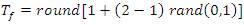
Tf : Teacher factor ranges from 1 to 2 using the equation:
Mi,j : Mean result of the learner in subject 'j'.
6. Calculate each learner,

where Xj,k,i : Result of learner “k” in Subject “j” and Xj,k,i ’ : Update of learner “k” in subject “j”.
7. Compare between two learners randomly ( P and Q)


8. For each subject, Repeat from step 5 to 7 till maximum number of iterations “p” or optimum solution are reached.
The objective function is required to minimize the error voltage which means better performance, faster response, and lower variation in terminal voltage of synchronous generator in AVR system. There are many performance criteria which are used to reach optimum solution. They are represented as follows [29].


ISE and IAE are characterized by small maximum overshoot (Mp ) and long settling time (Ts ) because they weight all errors p s equally (time independent). ITSE overcomes this problem, but it has a complex analytic formula and is time consuming [29]. The used objective function is ISE in all calculations.
All optimization technique’s operation is given as a flowchart shown in Figure 5. Optimization techniques (LUS, HAS, TLBO) differ only in the way to update the gain values. The objective function is calculated to minimize Integrated Square Error (ISE).

Figure 5. Flowchart of Methodology
The system under study is shown in Figure 4 and modeled using MATLAB/SIMULINK with the following parameters: KA =10, TA =0.1, KE =1, TE =0.4, KG =1, TG =1, KS =1, and TS =0.01.
The system model will be as shown in Figure 6.
The transfer function will be as follows [29]:
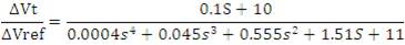

Figure 6. AVR System Model with the Parameters used in MATLAB
An AVR system without controller results in instability and slow response as shown in Figure 7 as used in MATLAB/SIMULINK when a step voltage of 1 p.u. is applied. The terminal voltage has slow response where Maximum overshoot is 1.507 p.u., Steady state error is 0.0881, rise time is 0.354 seconds, and settling time is 4.6 seconds.

Figure 7. Terminal Voltage without Controller in AVR System
In order to solve this problem, a controller is used to get faster response. PID and PIDA controllers are used. The controller is tuned by any optimization technique. Each controller is optimized by TLBO, HSA, and LUS.
Maximum iteration of all optimization techniques is adjusted to 100. TLBO and HSA are set to 100 populations. ISE is used as the objective function.
PID controller has three design variables or dimensions (Kp , Ki, Kd ). They range from zero to one.
Table 1 shows the performance of the three optimization techniques using PID controller. The table shows better response (lower overshoot, rise time, settling time, and steady state error) than using the AVR system without a controller. Figure 8 shows the terminal voltage of the three optimization techniques that improves the response of the AVR system when a step voltage of 1 p.u. is applied.
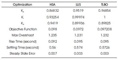
Table 1. Three Optimization Techniques using PID Controller in AVR System
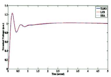
Figure 8. Terminal Voltage using PID Controller
Table 2 compares these results with MOL, GSA, ABC, PSO, and DE which are used in previous works using a PID controller in AVR system. This comparison shows that TLBO, LUS, and HSA have better response (lower overshoot, rise time, and settling time) than MOL, GSA, ABC, PSO, and DE. Figure 9 shows the terminal voltage of different optimization techniques using a PID controller in the AVR system when a step voltage of 1 p.u. is applied.

Table 2. Comparison with other Optimization Techniques using PID Controller
PIDA controller has six design variables (dimensions) used in the three used optimization techniques with ranges as follows [30, 32].

Figure 9. Terminal Voltage of different Optimization Techniques using PID Controller

Table 3 shows the performance of the three used optimization techniques. The table shows better response (lower overshoot, rise time, settling time, and steady state error) than using the AVR system without a controller. It also shows that TLBO has the best response compared to HSA and LUS which is the least. Figure 10 shows the three terminal voltages of the three optimization techniques when a step voltage of 1 p.u. is applied.

Table 3. Three Optimization Techniques using PIDA Controller in AVR System

Figure 10. Terminal Voltage using PIDA Controller
Table 4 shows a comparison between the three techniques and other optimization techniques BAT, CS, GA, and TS which are used in previous works using PIDA controller in AVR system. TLBO, HSA, and LUS show better performance and response (lower overshoot, rise time, and settling time) than BAT, CS, GA, and TS. Figure 11 shows the terminal voltage of different optimization techniques using PIDA controller in the AVR system when a step voltage of 1 p.u. is applied.
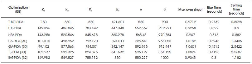
Table 4. Comparison with other Optimization Techniques using PIDA Controller
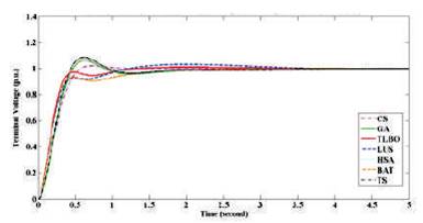
Figure 11. Terminal Voltage of different Optimization Techniques using PIDA Controller
AVR system has slow response without using controller due to load variation and the inductance of field windings. The controller is used to get faster response and optimization technique is used to tune the controller parameters. PID and PIDA controllers are used. Each is being optimized by TLBO, LUS, and HSA. For PID controller, they show better performance and response compared to MOL, GSA, ABC, PSO, and DE. For PIDA controller, they show better performance and response compared to BAT, CS, TS, and GA. By comparing both controllers, PIDA controller is better in maximum overshoot and steady state error than PID controller. On the other hand, PID controller is better in rise time and settling time than PIDA. As the used objective function is ISE, which is characterized by its bad setting time and rise time because it weights all errors equally (time independent). Consequently, PIDA controller has better response and performance than PID controller. So the best system used is TLBO-PIDA with the lowest overshoot and the best steady state error, then HSA-PIDA and the last but not least is LUS-PIDA.