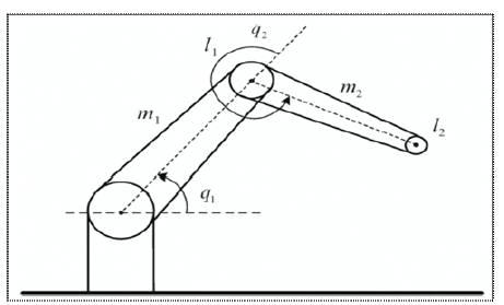
Figure 1. Two-link Robotic manipulator
Robotic manipulators have been extensively used in the industrial applications such as paint spraying, welding, accurate positioning system etc. where joint angles of robotic manipulators are directed to follow some given trajectories as close as possible. Therefore, trajectory tracking problem of robotic manipulators is the most significant and fundamental task for researchers to work upon. Robotic manipulator systems are inevitably subject to structured and unstructured uncertainties resulting in imprecision of its dynamical models and it is difficult to obtain a suitable mathematical model for the robotic control scheme. Robotic manipulators are dynamically coupled, multi-inputmulti- output, non-linear and time variant complex systems. This paper presents the dynamics of two link robotic manipulator. In this paper, PID (Proportional Integral Derivative), CTC (Computed Torque Control), SMC (Sliding Mode Control) and RBFNN (Radial Basis Function Neural Network) controllers are designed and implemented to the joint position control of two link robotic manipulators for pre-defined trajectory tracking control. Simulated results for different controllers are compared to show reduction in tracking error and performance improvement of two link robotic manipulators. Tracking performance and error comparison graphs are presented to demonstrate the performance of the proposed controllers. Further, comparison between chattering of SMC and RBFNN-SMC for joint 1 and joint 2 is also shown. The simulation work is carried out in MATLAB environment.
A robot is an electromechanical device which is guided by computer or electronic programming and is thus able to do tasks on its own. Robots have replaced slaves in the assistance of performing those repetitive and dangerous tasks which humans prefer not to do or unable to do due to size limitations or even those such as in outer space or at the bottom of the sea where humans could not survive the extreme environments. The control of a robot involves three distinct phases: a) Perception, b) Processing and c) Action. The robot control problem is typically decomposed hierarchically into two tasks such as motion control i.e. (trajectory tracking) and path planning.
Manipulators are multi-input-multi-output, non-linear and time variant complex systems [1]. Different types of controllers can be used to control the tracking path of robotic manipulators. PID controller is a conventional model free feedback control approach and has been extensively applied in industrial application because of its simplicity, easy to implement in hardware or software and does not require a precise process model to start up and maintain [2]. The principle objective of “Computed Torque Controllers (CTC) is to linearize and decouple the dynamical equations of motion so that each joint can be considered independently. Computed Torque Control (CTC) allows the design of considerably more precise, energy efficient, lower feedback gains and complaint controls for robots [3]. The main reason to select SMC is to have an acceptable control performance and solve the two most important challenging issues i.e stability and robustness in control [4]. So, there is a need for model-free adaptive control strategies such as control techniques based on soft computing methods i.e Neural [5]. Design procedure for the PID Controller does not require the knowledge of the robot dynamics, whereas CTC allows the design to be more precise, energy efficient, with lower feedback gain [6]. Due to the various drawbacks of CTC, robotics control was turned towards the more advanced techniques like SMC and Neural Network. This paper presents the comparative analysis of PID, CTC, SMC and RBFNN controllers which shows that performance of robotic manipulator using RBFNN controller is better than PID, CTC and SMC controllers [7].
The dynamic equations i.e a set of equations describing the dynamic behavior of the manipulator are useful for computer simulation of robot arm motion, the design of suitable control equations for a robot arm and the evaluation of the kinematic design and structure of a robot arm. Dynamic equations of the several types of manipulators, i.e. for two, three, five or n-links can be derived.The schematic of two link manipulator is shown in Figure 1.
Figure 1. Two-link Robotic manipulator
where l1 and l2 are the lengths; m1 and m2 are the mass of the links (joint 1 and joint 2 respectively), q1 is the angle of joint 1with respect to the inertial frame as depicted in Figure 1. The angle q2 of joint 2 is defined with respect to the orientation of the first link.
Dynamic model of a manipulator plays an important role for simulation of motion, analysis of manipulator structures and design of control algorithms. Simulating manipulator motion allows testing control strategies and motion planning techniques without the need to use a physically available system. Two problems related to manipulator dynamics are: Inverse dynamics in which the manipulator's equations of motion are solved for given motion to determine the generalized forces. Direct dynamics in which the equations of motion are integrated to determine the generalized coordinate response to applied generalized forces and are important to solve.
Various approaches are available to formulate robot arm dynamics, such as the Lagrange-Euler (L-E), the Newton- Euler, the recursive Lagrange-Euler, and the generalized d'Alembert principle formulations [1]. Deriving the dynamic model of a manipulator using the L-E method is simple and systematic. The resultant equations of motion, excluding the dynamics of the electronic control device and the gear friction, are a set of second order, coupled nonlinear differential equations. One approach that has the advantage of both speed and accuracy is based on the N-E vector formulation [3]. The derivation is simple, although messy, and involves vector cross-product terms. The resultant dynamic equations, excluding the dynamics of the control device and the gear friction, are a set of forward and backward recursive equations. These equations can be applied to the robot links sequentially.
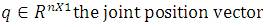
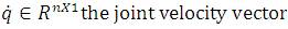
Using the Lagrangian formulation, the dynamic equation of an n - degree-of-freedom rigid manipulator can be expressed as [8]
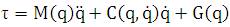
Where

G(q) includes the gravitational forces
M(q) the inertia matrix which is symmetric and positive definite;

τ represents the external torque to be applied on the manipulator by the actuators to control the angles q1 and q2 . The dynamic model is represented by equation 1, characterizing the behavior of robot manipulators in general and is composed of nonlinear functions of the state variables (joint positions and velocities). This feature of the dynamic model might lead us to believe that given any controller, the differential equation that models the control system in closed loop should also be composed of nonlinear functions of the corresponding state variables. Nevertheless, there exists a controller which is also nonlinear in the state variables, but which leads to a closed-loop control system which is described by a linear differential equation.
In order to control the arms (joint 1 and joint 2) of robotic manipulator, the torque at each joint must be calculated every moment. But with the increase of degree of freedom, calculating time also increases. Moreover, the unknown external forces also can be applied to the robot. Noh and Won [4] used a disturbance observer to find the effect of unknown forces like friction and damping effects. Different types of controllers can be used to improve the tracking performance of joint 1 and joint 2 of robotic manipulator.
PD/PID controllers are only capable of measuring varying inputs and calculating the difference between them. Hence, there is a need of more accurate and flexible model which can be used up with the time varying, nonlinear, complex system of today. The block diagram of PID controller is shown in Figure 2.
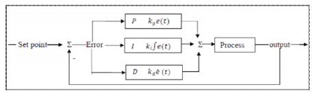
Figure 2. PID Controller
Torque equation for PD/PID controller is [9]
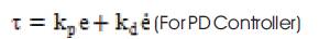

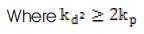
kp , kd and ki are the proportional controller gain, derivative controller gain and integral controller gain respectively.
In order to overcome the drawbacks of the PD controller, a more sophisticated scheme is Computed Torque Control (CTC) in which the magnitude of the nonlinear disturbing and loading torques is computed using the dynamic equations and is used to compensate the disturbances by means of a feed forward technique. The block diagram of computed-torque controlled robot manipulator is shown in Figure 3.
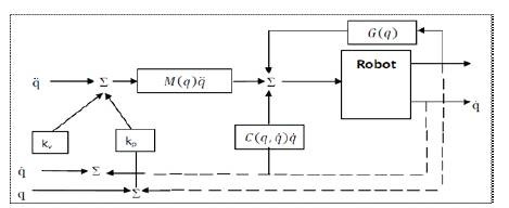
Figure 3. Computed Torque Controlled Robotic manipulator
The principle objective of Computed Torque Controller is to linearize and decouple the dynamical equations of motion so that each joint can be considered independently. CTC requires a considerable computed load since the torque has to be computed on-line so that the closed-loop system equations become linear and autonomous [8]. So, there is a need of a controller which is model independent and affected by parameter variation of robot model. Torque equation for CTC is given as [10-12].

Where gains kp and kv are chosen to meet some specific properties of the system and these gains should be adjusted to reduce the errors [11].
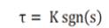
Sliding Mode Control (SMC) is a nonlinear control method which alters the dynamics of a nonlinear system by application of a discontinuous control signal that forces the system to "slide" along a cross-section of the system's normal behavior. The state-feedback control law is not a continuous function of time. Instead, it can switch from one continuous structure to another based on the current position in the state space. Sliding mode control is a variable structure control method. The multiple control structures are designed so that trajectories always move toward an adjacent region with a different control structure and so the ultimate trajectory will not exist entirely within one control structure. Instead, it will slide along the boundaries of the control structures. The motion of the system as it slides along these boundaries is called a sliding mode and the geometrical locus consisting of the boundaries is called the sliding (hyper) surface. In the context of modern control theory, any variable structure system like a system under SMC may be viewed as a special case of a hybrid dynamical system as the system not only flows through a continuous state space but also moves through different discrete control modes. In fact, although the system is nonlinear, in general, the idealized (i.e., non-chattering) behavior of the system when confined to the surface is an LTI (Linear Time Invariant) system with an exponentially stable origin. Torque equation for SMC controller is [11].

Block diagram of robotic manipulator using SMC is shown in Figure 4.
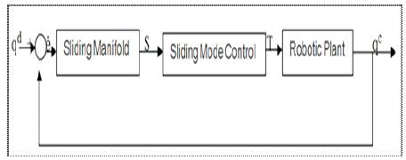
Figure 4. Sliding Mode Controlled Robotic Manipulator
Intuitively, sliding mode control uses practically infinite gain to force the trajectories of a dynamic system to slide along the restricted sliding mode subspace. Trajectories from this reduced-order sliding mode have desirable properties (e.g., the system naturally slides along it until it comes to rest at a desired equilibrium). The main strength of sliding mode control is its robustness. Because the control can be as simple as a switching between two states (e.g., "on"/"off" or "forward"/"reverse"), it need not be precise and will not be sensitive to parameter variations that enter into the control channel. Additionally, because the control law is not a continuous function, the sliding mode can be reached in finite time.
SMC has two problems: Chattering problem and sensitivity. Firstly Chattering problem causes the high frequency oscillations of the controllers output. Chattering phenomenon can cause some problems such as saturation and heat for mechanical parts of robot manipulators or drivers. To reduce the chattering, various papers have been reported by many researchers and classified into two most important methods, namely, boundary layer saturation method and estimated uncertainties method. Secondly, sensitivity, this controller is very sensitive to the noise when the input signals are very close to zero.
Neural network or simply an Artificial Neural Network(ANN) is a software application that alters certain variables in response to a set of corresponding input and output patterns. Beginning with an initial set of internal values, the network modifies these quantities in order to find a position of “best fit,” thereby generating from the input patterns their expected results.
The basic model of multi-layer neural networks utilizes either sigmoid or threshold neurons. These threshold logic units (TLUs) generate a signal, or “fire,” when the sum of their input signals exceeds a certain level. Sigmoid units provide a more graceful degradation of output signals and because the derivative of this function can be taken the back propagation method, which relies on this value, can be implemented for training purposes.
Radial Basis Function (RBF) neural networks operate on a somewhat different principle. Instead of having threshold units with a single value against which is to compare accumulated sums of input signals, each RBF neuron has a set of values called a“reference vector” for comparison with an input set of the same cardinality. The driving formula of each neuron used in this paper is the multivariate Gaussian function:
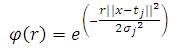
Where x is the input vector for the neuron, tj is the set of reference values, j is the standard deviation and (σ2 is the variance) of the function for each of the centers (j) and the value r (||x - tj||) is the Euclidean distance between a center vector and the set of data points. The most common architecture for an RBF neural network is the fully connected single hidden layer arrangement as shown in Figure 5.
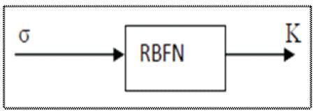
Figure 5. Block diagram of Radial Basis Function Neural Network (RBFNN)
In such an arrangement, each of the neurons of the hidden layer operate on the Gaussian formula given by equation 9, comparing a reference vector of a length equal to the number of inputs. The output layer in this case consists of a single neuron, although radial basis networks are fully capable of supporting numerous such units and is defined by a linear function of the hidden units' values.
In an RBF network, each of the hidden neurons contains a complete reference vector corresponding to the number of inputs. Each comparison between the input vector and these reference vectors represents a dimension for use by the output layer in determining classification. When the number of neurons is equivalent to the cardinality of the input vector, each neuron may be used to respond to a single pattern of inputs. While this is ideal where there are limited, finite input patterns, a network that has become familiar with the input variables to this degree is often not optimal for continuous data. If a network perfectly classifies the training data, yet is unable to accurately recognize the patterns when provided with new but similar input patterns, the system is described as being over trained. This overtraining effect known as “over fitting,” results from a loss of generality. The neurons become un-trained to precise patterns of information, focusing on non-generic aspects of the training set, and are therefore unable to recognize those sets of data which deviate in the slightest manner from the sequences on which it was trained [13] .
The obvious remedy to this problem is to reduce the number of hidden units and the selection of the number of neurons in a given network is therefore an important aspect of its architecture. The methods employed in order to train such a reduced neuron system are based upon the properties of Green's functions, which allow a process of supervised selection of centers to regulate the variables within the reference vectors of those neurons. The Gaussian function takes advantage of approximation techniques (discussed below), in which each neuron is able to identify multiple patterns, which are further differentiated by the output layers. An exposition of the approximation techniques based upon Gaussian properties is provided by Haykin [14].
The 'learning' capability of the NN is exploited for learning non-linear function representing direct dynamics, inverse dynamics and other characteristics of the system. Learning can be done off-line and needs no data recording of actual operation. Architecture for an RBFN network has 3 layers namely Input layer, Hidden layer and Output layer. A general structure of a RBFN is given in Figure 6.
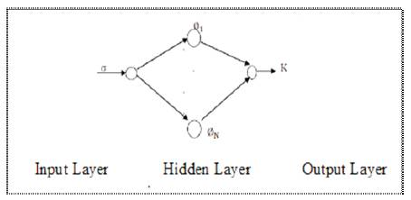
Figure 6. Basic structure of RBFNN
The input neurons (or processing before the input layer) standardize the range of the values by subtracting the median and dividing by the interquartile range. The input neurons then feed the values to each of the neurons in the hidden layer.
Hidden layer has a variable number of neurons (the optimal number is determined by the training process). Each neuron consists of a radial basis function centered on a point with as many dimensions as there are predictor variables. The spread (radius) of the RBF function may be different for each dimension. The centers and spreads are determined by the training process. When presented with the x vector of input values from the input layer, a hidden neuron computes the Euclidean distance of the test case from the neuron's center point and then applies the RBF kernel function to this distance using the spread values. The resulting value is passed to the summation layer. The value coming out of a neuron in the hidden layer is multiplied by a weight associated with the neurons and passed to the summation which adds up the weighted values and presents this sum as the output of the network. For classification problems, there is one output (and a separate set of weights and summation unit) for each target category. The value output for a category is the probability that the case being evaluated has that category.
Various methods have been used to train RBF networks. One approach first uses K-means clustering to find cluster centers which are then used as the centers for the RBF functions. However, K-mean sclustering is a computationally intensive procedure, and it often does not generate the optimal number of centers. This algorithm uses an evolutionary approach to determine the optimal center points and spreads for each neuron. The computation of the optimal weights between the neurons in the hidden layer and the summation layer is done using ridge regression.
In this paper, four controllers PID, CTC, SMC and RBFNN [13- 16)]are proposed for robotic manipulator. All these controllers are implemented on two link robotic manipulator. To illustrate the performance of proposed models, robotic manipulator using these controllers have been simulated on MATLAB. General flow chart for implementation of different controllers and calculation of various parameters/gains of controllers is given by flow chart shown in Figure 7. Input to the robotic manipulator is pre -defined path trajectory which must be followed by it.
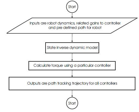
Figure 7. General flowchart for simulation of different controllers
Output results have been calculated and analyzed using graphs of simulated results. Controllers are tuned using Trial and error method. Comparison for the path trajectory of different controllers for joint 1 and joint 2 are shown in Figures 8 and 9 respectively. Errors of different controllers with the pre-defined path of robot in the form of graph are shown in Figures 10, and 11. Chattering between joint 1 and joint 2 are compared for SMC and RBFNN-SMC controller and is shown in Figures 12 and 13 respectively.
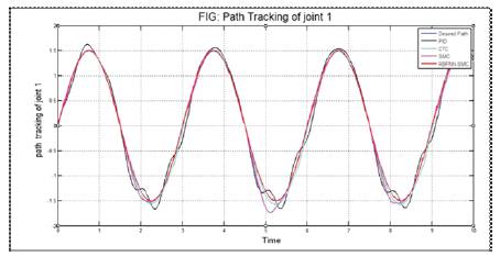
Figure 8. Comparison of path trajectory of different controller for joint 1 with desired path.
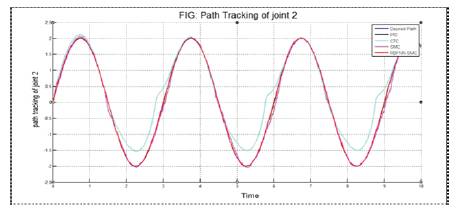
Figure 9. Comparison of path trajectory of different controllers for joint 2 with desired path
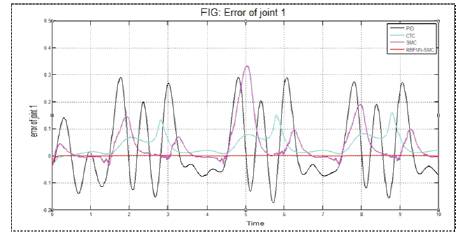
Figure 10. Comparison of error of different controllers for joint 1
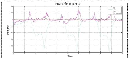
Figure 11. Comparison of error of different controllers for joint 2
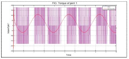
Figure 12. Comparison of chattering between SMC and RBFNN-SMC for joint 1
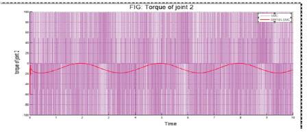
Figure 13. Comparison of chattering between SMC and RBFNN-SMC for joint 2
Based upon the simulated results, comparison of Mean Squared Normalized Error (MSE) for the path trajectory of robotic manipulator for different controllers is given in Table 1.
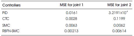
Table 1. MSE for tracking path of robotic manipulator using different controllers
In this paper, various control techniques such as PID, CTC, SMC schemes to upcoming intelligent NN, for path tracking of a two link robotic manipulator have been reviewed. Their merits and limitations have been discussed individually. Dynamic equations of two ink robotic manipulators have been derived. Due to the strong nonlinear characteristics and parameter variations in real environments, model based tracking control of robot manipulator is difficult. In this paper, PID, CTC, SMC and RBFNN Controllers to control the joint position of a two-link robot manipulator for achieving periodical and predefined trajectory tracking tasks has been presented. Tracking performance and error in tracking the desired trajectory using RBFNN controller has been compared with PID, CTC and SMC control schemes. As shown in Table 1,it has been found that tracking control of two link manipulator using RBFNN controller gives substantial improvement in path tracking as compared to the PID, CTC and SMC control. Further, using SMC based RBFNN, chattering problem has been drastically reduced as compared to SMC controller.